
 | ||
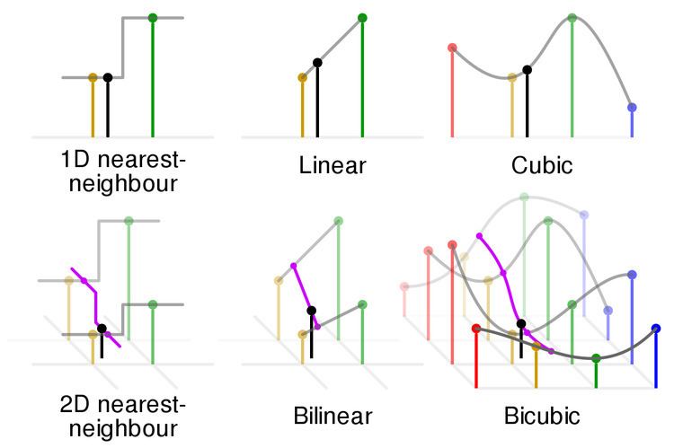
In mathematics, bicubic interpolation is an extension of cubic interpolation for interpolating data points on a two dimensional regular grid. The interpolated surface is smoother than corresponding surfaces obtained by bilinear interpolation or nearest-neighbor interpolation. Bicubic interpolation can be accomplished using either Lagrange polynomials, cubic splines, or cubic convolution algorithm.
Contents
- Computation
- Finding derivatives from function values
- Bicubic convolution algorithm
- Use in computer graphics
- References
In image processing, bicubic interpolation is often chosen over bilinear interpolation or nearest neighbor in image resampling, when speed is not an issue. In contrast to bilinear interpolation, which only takes 4 pixels (2×2) into account, bicubic interpolation considers 16 pixels (4×4). Images resampled with bicubic interpolation are smoother and have fewer interpolation artifacts.
Computation
Suppose the function values
The interpolation problem consists of determining the 16 coefficients
-
f ( 0 , 0 ) = p ( 0 , 0 ) = a 00 -
f ( 1 , 0 ) = p ( 1 , 0 ) = a 00 + a 10 + a 20 + a 30 -
f ( 0 , 1 ) = p ( 0 , 1 ) = a 00 + a 01 + a 02 + a 03 -
f ( 1 , 1 ) = p ( 1 , 1 ) = ∑ i = 0 3 ∑ j = 0 3 a i j
Likewise, eight equations for the derivatives in the
-
f x ( 0 , 0 ) = p x ( 0 , 0 ) = a 10 -
f x ( 1 , 0 ) = p x ( 1 , 0 ) = a 10 + 2 a 20 + 3 a 30 -
f x ( 0 , 1 ) = p x ( 0 , 1 ) = a 10 + a 11 + a 12 + a 13 -
f x ( 1 , 1 ) = p x ( 1 , 1 ) = ∑ i = 1 3 ∑ j = 0 3 a i j i -
f y ( 0 , 0 ) = p y ( 0 , 0 ) = a 01 -
f y ( 1 , 0 ) = p y ( 1 , 0 ) = a 01 + a 11 + a 21 + a 31 -
f y ( 0 , 1 ) = p y ( 0 , 1 ) = a 01 + 2 a 02 + 3 a 03 -
f y ( 1 , 1 ) = p y ( 1 , 1 ) = ∑ i = 0 3 ∑ j = 1 3 a i j j
And four equations for the cross derivative
-
f x y ( 0 , 0 ) = p x y ( 0 , 0 ) = a 11 -
f x y ( 1 , 0 ) = p x y ( 1 , 0 ) = a 11 + 2 a 21 + 3 a 31 -
f x y ( 0 , 1 ) = p x y ( 0 , 1 ) = a 11 + 2 a 12 + 3 a 13 -
f x y ( 1 , 1 ) = p x y ( 1 , 1 ) = ∑ i = 1 3 ∑ j = 1 3 a i j i j
where the expressions above have used the following identities,
This procedure yields a surface
Grouping the unknown parameters
and letting
the above system of equations can be reformulated into a matrix for the linear equation
Inverting the matrix gives the more useful linear equation
There can be another concise matrix form for 16 coefficients
Finding derivatives from function values
If the derivatives are unknown, they are typically approximated from the function values at points neighbouring the corners of the unit square, e.g. using finite differences.
To find either of the single derivatives,
To find the cross derivative,
At the edges of the dataset, when one is missing some of the surrounding points, the missing points can be approximated by a number of methods. A simple and common method is to assume that the slope from the existing point to the target point continues without further change, and using this to calculate a hypothetical value for the missing point.
Bicubic convolution algorithm
Bicubic spline interpolation requires the solution of the linear system described above for each grid cell. An interpolator with similar properties can be obtained by applying a convolution with the following kernel in both dimensions:
where
This approach was proposed by Keys who showed that
If we use the matrix notation for the common case
for
For two dimensions first applied once in
Use in computer graphics
The bicubic algorithm is frequently used for scaling images and video for display (see bitmap resampling). It preserves fine detail better than the common bilinear algorithm.
However, due to the negative lobes on the kernel, it causes overshoot (haloing). This can cause clipping, and is an artifact (see also ringing artifacts), but it increases acutance (apparent sharpness), and can be desirable.