In polynomial interpolation of two variables, the Padua points are the first known example (and up to now the only one) of a unisolvent point set (that is, the interpolating polynomial is unique) with minimal growth of their Lebesgue constant, proven to be O(log2 n) . Their name is due to the University of Padua, where they were originally discovered.
The points are defined in the domain [ − 1 , 1 ] × [ − 1 , 1 ] ⊂ R 2 . It is possible to use the points with four orientations, obtained with subsequent 90-degree rotations: this way we get four different families of Padua points.
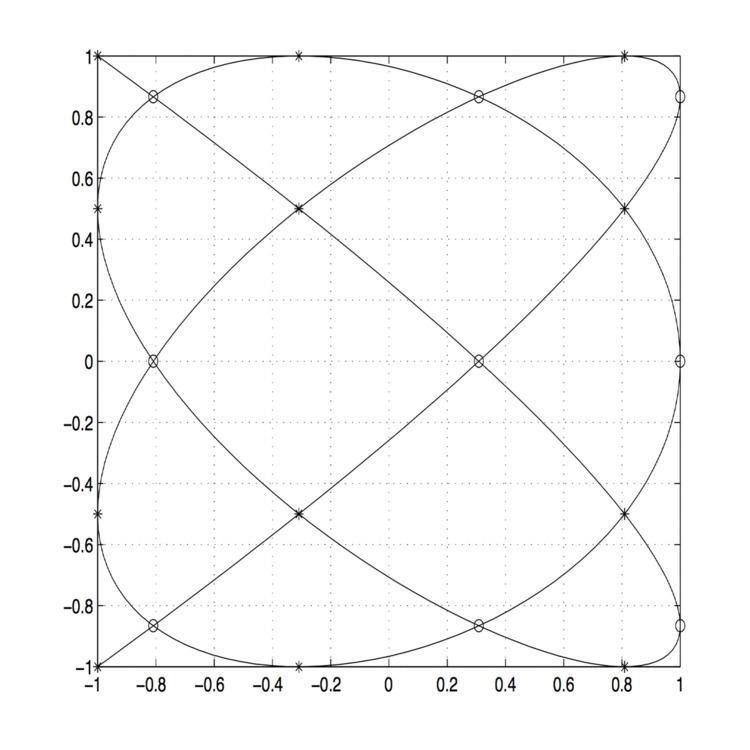
We can see the Padua point as a "sampling" of a parametric curve, called generating curve, which is slightly different for each of the four families, so that the points for interpolation degree n and family s can be defined as
Pad n s = { ξ = ( ξ 1 , ξ 2 ) } = { γ s ( k π n ( n + 1 ) ) , k = 0 , … , n ( n + 1 ) } . Actually, the Padua points lie exactly on the self-intersections of the curve, and on the intersections of the curve with the boundaries of the square [ − 1 , 1 ] 2 . The cardinality of the set Pad n s is | Pad n s | = N = ( n + 1 ) ( n + 2 ) 2 . Moreover, for each family of Padua points, two points lie on consecutive vertices of the square [ − 1 , 1 ] 2 , 2 n − 1 points lie on the edges of the square, and the remaining points lie on the self-intersections of the generating curve inside the square.
The four generating curves are closed parametric curves in the interval [ 0 , 2 π ] , and are a special case of Lissajous curves.
The generating curve of Padua points of the first family is
γ 1 ( t ) = [ − cos ( ( n + 1 ) t ) , − cos ( n t ) ] , t ∈ [ 0 , π ] . If we sample it as written above, we have:
Pad n 1 = { ξ = ( μ j , η k ) , 0 ≤ j ≤ n ; 1 ≤ k ≤ ⌊ n 2 ⌋ + 1 + δ j } , where δ j = 0 when n is even or odd but j is even, δ j = 1 if n and k are both odd
with
μ j = cos ( j π n ) , η k = { cos ( ( 2 k − 2 ) π n + 1 ) j odd cos ( ( 2 k − 1 ) π n + 1 ) j even. From this follows that the Padua points of first family will have two vertices on the bottom if n is even, or on the left if n is odd.
The generating curve of Padua points of the second family is
γ 2 ( t ) = [ − cos ( n t ) , − cos ( ( n + 1 ) t ) ] , t ∈ [ 0 , π ] , which leads to have vertices on the left if n is even and on the bottom if n is odd.
The generating curve of Padua points of the third family is
γ 3 ( t ) = [ cos ( ( n + 1 ) t ) , cos ( n t ) ] , t ∈ [ 0 , π ] , which leads to have vertices on the top if n is even and on the right if n is odd.
The generating curve of Padua points of the fourth family is
γ 4 ( t ) = [ cos ( n t ) , cos ( ( n + 1 ) t ) ] , t ∈ [ 0 , π ] , which leads to have vertices on the right if n is even and on the top if n is odd.
The explicit representation of their fundamental Lagrange polynomial is based on the reproducing kernel K n ( x , y ) , x = ( x 1 , x 2 ) and y = ( y 1 , y 2 ) , of the space Π n 2 ( [ − 1 , 1 ] 2 ) equipped with the inner product
⟨ f , g ⟩ = 1 π 2 ∫ [ − 1 , 1 ] 2 f ( x 1 , x 2 ) g ( x 1 , x 2 ) d x 1 1 − x 1 2 d x 2 1 − x 2 2 defined by
K n ( x , y ) = ∑ k = 0 n ∑ j = 0 k T ^ j ( x 1 ) T ^ k − j ( x 2 ) T ^ j ( y 1 ) T ^ k − j ( y 2 ) with T ^ j representing the normalized Chebyshev polynomial of degree j (that is, T ^ 0 = T 0 , T ^ p = 2 T p where T p ( ⋅ ) = cos ( p arccos ( ⋅ ) ) is the classical Chebyshev polynomial of first kind of degree p ). For the four families of Padua points, which we may denote by Pad n s = { ξ = ( ξ 1 , ξ 2 ) } , s = { 1 , 2 , 3 , 4 } , the interpolation formula of order n of the function f : [ − 1 , 1 ] 2 → R 2 on the generic target point x ∈ [ − 1 , 1 ] 2 is then
L n s f ( x ) = ∑ ξ ∈ Pad n s f ( ξ ) L ξ s ( x ) where L ξ s ( x ) is the fundamental Lagrange polynomial
L ξ s ( x ) = w ξ ( K n ( ξ , x ) − T n ( ξ i ) T n ( x i ) ) , s = 1 , 2 , 3 , 4 , i = 2 − ( s mod 2 ) . The weights w ξ are defined as
w ξ = 1 n ( n + 1 ) ⋅ { 1 2 if ξ is a vertex point 1 if ξ is an edge point 2 if ξ is an interior point.