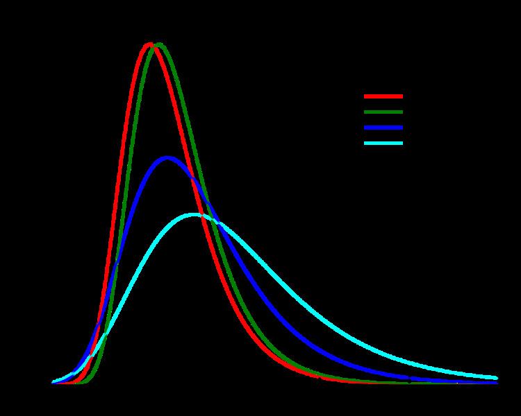
Gumbel distribution - Alchetron, The Free Social Encyclopedia



Parameters μ {\displaystyle \mu \!} location (real) β > 0 {\displaystyle \beta >0\!} scale (real) Support x ∈ ( − ∞ ; + ∞ ) {\displaystyle x\in (-\infty ;+\infty )\!} PDF 1 β e − ( z + e − z ) {\displaystyle {\frac {1}{\beta }}e^{-(z+e^{-z})}\!} where z = x − μ β {\displaystyle z={\frac {x-\mu }{\beta }}\!} CDF e − e − ( x − μ ) / β {\displaystyle e^{-e^{-(x-\mu )/\beta }}\!} Mean μ + β γ {\displaystyle \mu +\beta \,\gamma \!} where γ {\displaystyle \gamma } is Euler–Mascheroni constant Median μ − β ln ⁡ ( ln ⁡ ( 2 ) ) {\displaystyle \mu -\beta \,\ln(\ln(2))\!}

In probability theory and statistics, the Gumbel distribution (Generalized Extreme Value distribution Type-I) is used to model the distribution of the maximum (or the minimum) of a number of samples of various distributions. This distribution might be used to represent the distribution of the maximum level of a river in a particular year if there was a list of maximum values for the past ten years. It is useful in predicting the chance that an extreme earthquake, flood or other natural disaster will occur. The potential applicability of the Gumbel distribution to represent the distribution of maxima relates to extreme value theory, which indicates that it is likely to be useful if the distribution of the underlying sample data is of the normal or exponential type. The rest of this article refers to the Gumbel to model the distribution of the maximum value. To model the minimum value, use the negative of the original values.

The Gumbel distribution is a particular case of the generalized extreme value distribution (also known as the Fisher-Tippett distribution). It is also known as the log-Weibull distribution and the double exponential distribution (a term that is alternatively sometimes used to refer to the Laplace distribution). It is related to the Gompertz distribution: when its density is first reflected about the origin and then restricted to the positive half line, a Gompertz function is obtained.

In the latent variable formulation of the multinomial logit model — common in discrete choice theory — the errors of the latent variables follow a Gumbel distribution. This is useful because the difference of two Gumbel-distributed random variables has a logistic distribution.

The Gumbel distribution is named after Emil Julius Gumbel (1891–1966), based on his original papers describing the distribution.

Properties

The cumulative distribution function of the Gumbel distribution is

F ( x ; μ , β ) = e − e − ( x − μ ) / β .

The mode is μ, while the median is μ − β ln ⁡ ( ln ⁡ 2 ) , and the mean is given by

E ⁡ ( X ) = μ + γ β ,

where γ ≈ 0.5772 is the Euler–Mascheroni constant. The standard deviation is β π / 6 .

Standard Gumbel distribution

The standard Gumbel distribution is the case where μ = 0 and β = 1 with cumulative distribution function

F ( x ) = e − e ( − x )

and probability density function

f ( x ) = e − ( x + e − x ) .

In this case the mode is 0, the median is − ln ⁡ ( ln ⁡ ( 2 ) ) ≈ 0.3665 , the mean is γ , and the standard deviation is π / 6 ≈ 1.2825.

The cumulants, for n>1, are given by

κ n = ( n − 1 ) ! ζ ( n ) .

Quantile function and generating Gumbel variates

Since the quantile function(inverse cumulative distribution function), Q ( p ) , of a Gumbel distribution is given by

Q ( p ) = μ − β ln ⁡ ( − ln ⁡ ( p ) ) ,

the variate Q ( U ) has a Gumbel distribution with parameters μ and β when the random variate U is drawn from the uniform distribution on the interval ( 0 , 1 ) .

If X has a Gumbel distribution, then the conditional distribution of Y=-X given that Y is positive, or equivalently given that X is negative, has a Gompertz distribution. The cdf G of Y is related to F, the cdf of X, by the formula G ( y ) = P ( Y ≤ y ) = P ( X ≥ − y | X ≤ 0 ) = ( F ( 0 ) − F ( − y ) ) / F ( 0 ) for y>0. Consequently the densities are related by g ( y ) = f ( − y ) / F ( 0 ) : the Gompertz density is proportional to a reflected Gumbel density, restricted to the positive half-line.

If X is an exponential with mean 1, then -log(X) has a standard Gumbel-Distribution.

Theory related to the generalized multivariate log-gamma distribution provides a multivariate version of the Gumbel distribution.

Probability paper

In pre-software times probability paper was used to picture the Gumbel distribution (see illustration). The paper is based on linearization of the cumulative distribution function F :

− ln ⁡ [ − ln ⁡ ( F ) ] = ( x − μ ) / β

In the paper the horizontal axis is constructed at a double log scale. The vertical axis is linear. By plotting F on the horizontal axis of the paper and the x -variable on the vertical axis, the distribution is represented by a straight line with a slope 1 / β . When distribution fitting software like CumFreq became available, the task of plotting the distribution was made easier, as is demonstrated in the section below.

Notice for Wolfram MathWorld and MATLAB users

The Gumbel Distribution in Wolfram MathWorld and MATLAB is used to refer to the distribution corresponding to a minimum extreme value distribution which is not same with the Gumbel distribution in Wikipedia (which models the maximum); in this case to model the maximum value, use the negative of the original values, that is, the negative of x and the negative of the mode μ .

Application

Gumbel has shown that the maximum value (or last order statistic) in a sample of a random variable following an exponential distribution approaches the Gumbel distribution closer with increasing sample size.

In hydrology, therefore, the Gumbel distribution is used to analyze such variables as monthly and annual maximum values of daily rainfall and river discharge volumes, and also to describe droughts.

Gumbel has also shown that the estimator r/(n+1) for the probability of an event—where r is the rank number of the observed value in the data series and n is the total number of observations—is an unbiased estimator of the cumulative probability around the mode of the distribution. Therefore, this estimator is often used as a plotting position.

The blue picture illustrates an example of fitting the Gumbel distribution to ranked maximum one-day October rainfalls showing also the 90% confidence band based on the binomial distribution. The rainfall data are represented by the plotting position r/(n+1) as part of the cumulative frequency analysis.

In number theory, the Gumbel distribution approximates the number of terms in a partition of an integer as well as the trend-adjusted sizes of record prime gaps and record gaps between prime constellations.

In machine learning, the Gumbel distribution is sometimes employed to generate samples from the categorical distribution for example.

References

Gumbel distribution Wikipedia

(Text) CC BY-SA

Contents