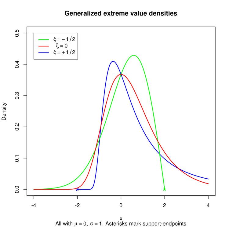
Generalized extreme value distribution - Alchetron, the free social encyclopedia



Notation GEV ( μ , σ , ξ ) {\displaystyle {\textrm {GEV}}(\mu ,\,\sigma ,\,\xi )} Parameters μ ∈ R — location, σ > 0 — scale, ξ ∈ R — shape. Support x ∈ [ μ − σ / ξ, +∞) when ξ > 0, x ∈ (−∞, +∞) when ξ = 0, x ∈ (−∞, μ − σ / ξ ] when ξ < 0. PDF 1 σ t ( x ) ξ + 1 e − t ( x ) , {\displaystyle {\frac {1}{\sigma }}\,t(x)^{\xi +1}e^{-t(x)},} where t ( x ) = { ( 1 + ξ ( x − μ σ ) ) − 1 / ξ if ξ ≠ 0 e − ( x − μ ) / σ if ξ = 0 {\displaystyle t(x)={\begin{cases}{\big (}1+\xi ({\tfrac {x-\mu }{\sigma }}){\big )}^{-1/\xi }&{\textrm {if}}\ \xi \neq 0\\e^{-(x-\mu )/\sigma }&{\textrm {if}}\ \xi =0\end{cases}}} CDF e − t ( x ) , {\displaystyle e^{-t(x)},\,} for x ∈ support Mean { μ + σ Γ ( 1 − ξ ) − 1 ξ if ξ ≠ 0 , ξ < 1 , μ + σ γ if ξ = 0 , ∞ if ξ ≥ 1 , {\displaystyle {\begin{cases}\mu +\sigma {\frac {\Gamma (1-\xi )-1}{\xi }}&{\text{if}}\ \xi \neq 0,\xi <1,\\\mu +\sigma \,\gamma &{\text{if}}\ \xi =0,\\\infty &{\text{if}}\ \xi \geq 1,\end{cases}}} where γ {\displaystyle \gamma } is Euler’s constant.

In probability theory and statistics, the generalized extreme value (GEV) distribution is a family of continuous probability distributions developed within extreme value theory to combine the Gumbel, Fréchet and Weibull families also known as type I, II and III extreme value distributions. By the extreme value theorem the GEV distribution is the only possible limit distribution of properly normalized maxima of a sequence of independent and identically distributed random variables. Note that a limit distribution need not exist: this requires regularity conditions on the tail of the distribution. Despite this, the GEV distribution is often used as an approximation to model the maxima of long (finite) sequences of random variables.

In some fields of application the generalized extreme value distribution is known as the Fisher–Tippett distribution, named after Ronald Fisher and L. H. C. Tippett who recognised three function forms outlined below. However usage of this name is sometimes restricted to mean the special case of the Gumbel distribution.

Specification

The generalized extreme value distribution has cumulative distribution function

F ( x ; μ , σ , ξ ) = exp ⁡ { − [ 1 + ξ ( x − μ σ ) ] − 1 / ξ }

for 1 + ξ ( x − μ ) / σ > 0 , where μ ∈ R is the location parameter, σ > 0 the scale parameter and ξ ∈ R the shape parameter. Thus for ξ > 0 , the expression just given for the cumulative distribution function is valid for x > μ − σ / ξ , while for ξ < 0 it is valid for x < μ + σ / ( − ξ ) . In the first case, at the lower end-point it equals 0; in the second case, at the upper end-point, it equals 1. For ξ = 0 the expression just given for the cumulative distribution function is formally undefined and is replaced by the result obtained by taking the limit as ξ → 0

F ( x ; μ , σ , 0 ) = exp ⁡ { − exp ⁡ [ − ( x − μ σ ) ] } ,

without any restriction on x.

The density function is, consequently,

f ( x ; μ , σ , ξ ) = 1 σ [ 1 + ξ ( x − μ σ ) ] ( − 1 / ξ ) − 1 exp ⁡ { − [ 1 + ξ ( x − μ σ ) ] − 1 / ξ }

again, for x > μ − σ / ξ in the case ξ > 0 , and for x < μ + σ / ( − ξ ) in the case ξ < 0 . The density is zero outside of the relevant range. In the case ξ = 0 the density is positive on the whole real line and equal to

f ( x ; μ , σ , 0 ) = 1 σ exp ⁡ [ − ( x − μ σ ) ] exp ⁡ { − exp ⁡ [ − ( x − μ σ ) ] } .

Since the cumulative distribution function is invertible, the quantile function for the GEV has an explicit expression, namely

Q ( p ; μ , σ , ξ ) = { μ + σ ( ( log ⁡ ( 1 / p ) ) − ξ − 1 ) / ξ ξ > 0 , then p ∈ ( 0 , 1 ] ; ξ < 0 , then p ∈ [ 0 , 1 ) μ + σ log ⁡ ( 1 / log ⁡ ( 1 / p ) ) ξ = 0 , p ∈ ( 0 , 1 ) .

Summary statistics

Some simple statistics of the distribution are:

E ⁡ ( X ) = μ − σ ξ + σ ξ g 1 for ξ < 1 Var ⁡ ( X ) = σ 2 ξ 2 ( g 2 − g 1 2 ) , Mode ⁡ ( X ) = μ + σ ξ [ ( 1 + ξ ) − ξ − 1 ] .

The skewness is for ξ>0

skewness ⁡ ( X ) = g 3 − 3 g 1 g 2 + 2 g 1 3 ( g 2 − g 1 2 ) 3 / 2

For ξ<0, the sign of the numerator is reversed.

The excess kurtosis is:

k u r t o s i s e x c e s s ⁡ ( X ) = g 4 − 4 g 1 g 3 + 6 g 2 g 1 2 − 3 g 1 4 ( g 2 − g 1 2 ) 2 − 3.

where g k = Γ ( 1 − k ξ ) , k=1,2,3,4, and Γ ( t ) is the gamma function.

Link to Fréchet, Weibull and Gumbel families

The shape parameter ξ governs the tail behavior of the distribution. The sub-families defined by ξ = 0 , ξ > 0 and ξ < 0 correspond, respectively, to the Gumbel, Fréchet and Weibull families, whose cumulative distribution functions are displayed below.

Gumbel or type I extreme value distribution ( ξ = 0 )

F ( x ; μ , σ , 0 ) = e − e − ( x − μ ) / σ for x ∈ R .

Fréchet or type II extreme value distribution, if ξ = α − 1 > 0 and y = 1 + ξ ( x − μ ) / σ

F ( x ; μ , σ , ξ ) = { e − y − α y > 0 0 y ≤ 0.

Reversed Weibull or type III extreme value distribution, if ξ = − α − 1 < 0 and y = − ( 1 + ξ ( x − μ ) / σ )

F ( x ; μ , σ , ξ ) = { e − ( − y ) α y < 0 1 y ≥ 0

Remark I: The theory here relates to maxima and the distribution being discussed is an extreme value distribution for maxima. A generalised extreme value distribution for minima can be obtained, for example by substituting (−x) for x in the distribution function, and subtracting from one: this yields a separate family of distributions.

Remark II: The ordinary Weibull distribution arises in reliability applications and is obtained from the distribution here by using the variable t = μ − x , which gives a strictly positive support - in contrast to the use in the extreme value theory here. This arises because the Weibull distribution is used in cases that deal with the minimum rather than the maximum. The distribution here has an addition parameter compared to the usual form of the Weibull distribution and, in addition, is reversed so that the distribution has an upper bound rather than a lower bound. Importantly, in applications of the GEV, the upper bound is unknown and so must be estimated while when applying the Weibull distribution the lower bound is known to be zero.

Remark III: Note the differences in the ranges of interest for the three extreme value distributions: Gumbel is unlimited, Fréchet has a lower limit, while the reversed Weibull has an upper limit. More precisely, Extreme Value Theory (Univariate Theory) describes which of the three is the limiting law according to the initial law X and in particular depending on its tail (e.g. maximum distribution of a heavy tailed law converges to Fréchet).

One can link the type I to types II and III the following way: if the cumulative distribution function of some random variable X is of type II, and with the positive numbers as support, i.e. F ( x ; 0 , σ , α ) , then the cumulative distribution function of ln ⁡ X is of type I, namely F ( x ; ln ⁡ σ , 1 / α , 0 ) . Similarly, if the cumulative distribution function of X is of type III, and with the negative numbers as support, i.e. F ( x ; 0 , σ , − α ) , then the cumulative distribution function of ln ⁡ ( − X ) is of type I, namely F ( x ; − ln ⁡ σ , 1 / α , 0 ) .

Link to logit models (logistic regression)

Multinomial logit models, and certain other types of logistic regression, can be phrased as latent variable models with error variables distributed as Gumbel distributions (type I generalized extreme value distributions). This phrasing is common in the theory of discrete choice models, which include logit models, probit models, and various extensions of them, and derives from the fact that the difference of two type-I GEV-distributed variables follows a logistic distribution, of which the logit function is the quantile function. The type-I GEV distribution thus plays the same role in these logit models as the normal distribution does in the corresponding probit models.

Properties

The cumulative distribution function of the generalized extreme value distribution solves the stability postulate equation. The generalized extreme value distribution is a special case of a max-stable distribution, and is a transformation of a min-stable distribution.

Applications

The GEV distribution is widely used in the treatment of "tail risks" in fields ranging from insurance to finance. In the latter case, it has been considered as a means of assessing various financial risks via metrics such as Value at Risk.

However, the resulting shape parameters have been found to lie in the range leading to undefined means and variances, which underlines the fact that reliable data analysis is often impossible.

If X ∼ GEV ( μ , σ , 0 ) then m X + b ∼ GEV ( m μ + b , m σ , 0 )

If X ∼ Gumbel ( μ , σ ) (Gumbel distribution) then X ∼ GEV ( μ , σ , 0 )

If X ∼ Weibull ( σ , μ ) (Weibull distribution) then μ ( 1 − σ l o g X σ ) ∼ GEV ( μ , σ , 0 )

If X ∼ GEV ( μ , σ , 0 ) then σ exp ⁡ ( − X − μ μ σ ) ∼ Weibull ( σ , μ ) (Weibull distribution)

If X ∼ Exponential ( 1 ) (Exponential distribution) then μ − σ log ⁡ X ∼ GEV ( μ , σ , 0 )

If X ∼ G E V ( α , β , 0 ) and Y ∼ G E V ( α , β , 0 ) then X − Y ∼ L o g i s t i c ( 0 , β ) (Logistic distribution)

If X ∼ G E V ( α , β , 0 ) and Y ∼ G E V ( α , β , 0 ) then X + Y ∼ L o g i s t i c ( 2 α , β )

References

Generalized extreme value distribution Wikipedia

(Text) CC BY-SA

Contents