In numerical analysis, a branch of applied mathematics, the midpoint method is a one-step method for numerically solving the differential equation,
                              y          ′                (        t        )        =        f        (        t        ,        y        (        t        )        )        ,                y        (                  t                      0                          )        =                  y                      0                                  .
The explicit midpoint method is given by the formula
                              y                      n            +            1                          =                  y                      n                          +        h        f                  (                      t                          n                                +                                    h              2                                ,                      y                          n                                +                                    h              2                                f          (                      t                          n                                ,                      y                          n                                )          )                ,                        (        1        e        )                the implicit midpoint method by
                              y                      n            +            1                          =                  y                      n                          +        h        f                  (                      t                          n                                +                                    h              2                                ,                                    1              2                                (                      y                          n                                +                      y                          n              +              1                                )          )                ,                        (        1        i        )                for                     n        =        0        ,        1        ,        2        ,        …                 Here,                     h                 is the step size — a small positive number,                               t                      n                          =                  t                      0                          +        n        h        ,                 and                               y                      n                                   is the computed approximate value of                     y        (                  t                      n                          )        .                 The explicit midpoint method is also known as the modified Euler method, the implicit method is the most simple collocation method, and, applied to Hamiltionian dynamics, a symplectic integrator.
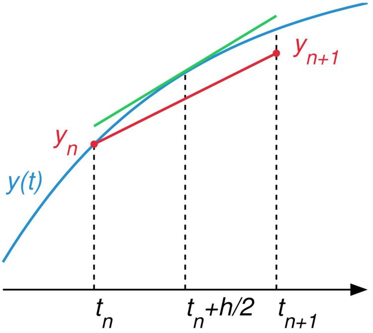
The name of the method comes from the fact that in the formula above the function                     f                 giving the slope of the solution is evaluated at                     t        =                  t                      n                          +        h                  /                2        ,                 (note :                     t                 is                                                                         t                                  n                                            +                              t                                  n                  +                  1                                                      2                                  ) which is the midpoint between                               t                      n                                   at which the value of y(t) is known and                               t                      n            +            1                                   at which the value of y(t) needs to be found.
The local error at each step of the midpoint method is of order                     O                  (                      h                          3                                )                        , giving a global error of order                     O                  (                      h                          2                                )                        . Thus, while more computationally intensive than Euler's method, the midpoint method's error generally decreases faster as                     h        →        0                .
The methods are examples of a class of higher-order methods known as Runge-Kutta methods.
The midpoint method is a refinement of the Euler's method
                              y                      n            +            1                          =                  y                      n                          +        h        f        (                  t                      n                          ,                  y                      n                          )        ,                        and is derived in a similar manner. The key to deriving Euler's method is the approximate equality
                    y        (        t        +        h        )        ≈        y        (        t        )        +        h        f        (        t        ,        y        (        t        )        )                        (        2        )                which is obtained from the slope formula
                              y          ′                (        t        )        ≈                                            y              (              t              +              h              )              −              y              (              t              )                        h                                          (        3        )                and keeping in mind that                               y          ′                =        f        (        t        ,        y        )        .                
For the midpoint methods, one replaces (3) with the more accurate
                              y          ′                          (          t          +                                    h              2                                )                ≈                                            y              (              t              +              h              )              −              y              (              t              )                        h                                  when instead of (2) we find
                    y        (        t        +        h        )        ≈        y        (        t        )        +        h        f                  (          t          +                                    h              2                                ,          y                      (            t            +                                          h                2                                      )                    )                .                        (        4        )                One cannot use this equation to find                     y        (        t        +        h        )                 as one does not know                     y                 at                     t        +        h                  /                2                . The solution is then to use a Taylor series expansion exactly as if using the Euler method to solve for                     y        (        t        +        h                  /                2        )                :
                    y                  (          t          +                                    h              2                                )                ≈        y        (        t        )        +                              h            2                                    y          ′                (        t        )        =        y        (        t        )        +                              h            2                          f        (        t        ,        y        (        t        )        )        ,                which, when plugged in (4), gives us
                    y        (        t        +        h        )        ≈        y        (        t        )        +        h        f                  (          t          +                                    h              2                                ,          y          (          t          )          +                                    h              2                                f          (          t          ,          y          (          t          )          )          )                        and the explicit midpoint method (1e).
The implicit method (1i) is obtained by approximating the value at the half step                     t        +        h                  /                2                 by the midpoint of the line segment from                     y        (        t        )                 to                     y        (        t        +        h        )                
                    y                  (          t          +                                    h              2                                )                ≈                              1            2                                                (                          y        (        t        )        +        y        (        t        +        h        )                              )                                  and thus
                                                        y              (              t              +              h              )              −              y              (              t              )                        h                          ≈                  y          ′                          (          t          +                                    h              2                                )                ≈        k        =        f                  (          t          +                                    h              2                                ,                                    1              2                                                          (                                y          (          t          )          +          y          (          t          +          h          )                                    )                                )                        Inserting the approximation                               y                      n                          +        h                k                 for                     y        (                  t                      n                          +        h        )                 results in the implicit Runge-Kutta method
                                                                        k                                                            =                f                                  (                                      t                                          n                                                        +                                                            h                      2                                                        ,                                      y                                          n                                                        +                                                            h                      2                                                        k                  )                                                                                                      y                                      n                    +                    1                                                                                              =                                  y                                      n                                                  +                h                                k                                                            which contains the implicit Euler method with step size                     h                  /                2                 as its first part.
Because of the time symmetry of the implicit method, all terms of even degree in                     h                 of the local error cancel, so that the local error is automatically of order                                           O                          (                  h                      3                          )                . Replacing the implicit with the explicit Euler method in the determination of                     k                 results again in the explicit midpoint method.