Bounded variation

History

According to Boris Golubov, BV functions of a single variable were first introduced by Camille Jordan, in the paper (Jordan 1881) dealing with the convergence of Fourier series. The first successful step in the generalization of this concept to functions of several variables was due to Leonida Tonelli, who introduced a class of continuous BV functions in 1926 (Cesari 1986, pp. 47–48), to extend his direct method for finding solutions to problems in the calculus of variations in more than one variable. Ten years after, in (Cesari 1936), Lamberto Cesari changed the continuity requirement in Tonelli's definition to a less restrictive integrability requirement, obtaining for the first time the class of functions of bounded variation of several variables in its full generality: as Jordan did before him, he applied the concept to resolve of a problem concerning the convergence of Fourier series, but for functions of two variables. After him, several authors applied BV functions to study Fourier series in several variables, geometric measure theory, calculus of variations, and mathematical physics. Renato Caccioppoli and Ennio de Giorgi used them to define measure of nonsmooth boundaries of sets (see the entry "Caccioppoli set" for further information). Olga Arsenievna Oleinik introduced her view of generalized solutions for nonlinear partial differential equations as functions from the space BV in the paper (Oleinik 1957), and was able to construct a generalized solution of bounded variation of a first order partial differential equation in the paper (Oleinik 1959): few years later, Edward D. Conway and Joel A. Smoller applied BV-functions to the study of a single nonlinear hyperbolic partial differential equation of first order in the paper (Conway & Smoller 1966), proving that the solution of the Cauchy problem for such equations is a function of bounded variation, provided the initial value belongs to the same class. Aizik Isaakovich Vol'pert developed extensively a calculus for BV functions: in the paper (Vol'pert 1967) he proved the chain rule for BV functions and in the book (Hudjaev & Vol'pert 1985) he, jointly with his pupil Sergei Ivanovich Hudjaev, explored extensively the properties of BV functions and their application. His chain rule formula was later extended by Luigi Ambrosio and Gianni Dal Maso in the paper (Ambrosio & Dal Maso 1990).

BV functions of one variable

Definition 1.1. The total variation of a real-valued (or more generally complex-valued) function f, defined on an interval [a, b]⊂ℝ is the quantity

where the supremum is taken over the set P = { P = { x 0 , … , x n P } | P  is a partition of  [ a , b ] } of all partitions of the interval considered.

If f is differentiable and its derivative is Riemann-integrable, its total variation is the vertical component of the arc-length of its graph, that is to say,

Definition 1.2. A real-valued function f on the real line is said to be of bounded variation (BV function) on a chosen interval [a, b]⊂ℝ if its total variation is finite, i.e.

It can be proved that a real function ƒ is of bounded variation in [ a , b ] if and only if it can be written as the difference ƒ = ƒ₁ − ƒ₂ of two non-decreasing functions on [ a , b ] : this result is known as the Jordan decomposition of a function and it is related to the Jordan decomposition of a measure.

Through the Stieltjes integral, any function of bounded variation on a closed interval [a, b] defines a bounded linear functional on C([a, b]). In this special case, the Riesz representation theorem states that every bounded linear functional arises uniquely in this way. The normalised positive functionals or probability measures correspond to positive non-decreasing lower semicontinuous functions. This point of view has been important in spectral theory, in particular in its application to ordinary differential equations.

BV functions of several variables

Functions of bounded variation, BV functions, are functions whose distributional derivative is a finite Radon measure. More precisely:

Definition 2.1. Let Ω be an open subset of ℝⁿ. A function u belonging to L 1 ( Ω ) is said of bounded variation (BV function), and written

if there exists a finite vector Radon measure D u ∈ M ( Ω , R n ) such that the following equality holds

that is, u defines a linear functional on the space C c 1 ( Ω , R n ) of continuously differentiable vector functions ϕ of compact support contained in Ω : the vector measure D u represents therefore the distributional or weak gradient of u .

An equivalent definition is the following.

Definition 2.2. Given a function u belonging to L 1 ( Ω ) , the total variation of u in Ω is defined as

where ∥ ∥ L ∞ ( Ω ) is the essential supremum norm. Sometimes, especially in the theory of Caccioppoli sets, the following notation is used

in order to emphasize that V ( u , Ω ) is the total variation of the distributional / weak gradient of u . This notation reminds also that if u is of class C 1 (i.e. a continuous and differentiable function having continuous derivatives) then its variation is exactly the integral of the absolute value of its gradient.

The space of functions of bounded variation (BV functions) can then be defined as

The two definitions are equivalent since if V ( u , Ω ) < + ∞ then

therefore ϕ ↦ ∫ Ω u ( x ) d i v ϕ ( x ) d x defines a continuous linear functional on the space C c 1 ( Ω , R n ) . Since C c 1 ( Ω , R n ) ⊂ C 0 ( Ω , R n ) as a linear subspace, this continuous linear functional can be extended continuously and linearily to the whole C 0 ( Ω , R n ) by the Hahn–Banach theorem. Hence the continuous linear functional defines a Radon measure by the Riesz-Markov Theorem.

Locally BV functions

If the function space of locally integrable functions, i.e. functions belonging to L l o c 1 ( Ω ) , is considered in the preceding definitions 1.2, 2.1 and 2.2 instead of the one of globally integrable functions, then the function space defined is that of functions of locally bounded variation. Precisely, developing this idea for definition 2.2, a local variation is defined as follows,

for every set U ∈ O c ( Ω ) , having defined O c ( Ω ) as the set of all precompact open subsets of Ω with respect to the standard topology of finite-dimensional vector spaces, and correspondingly the class of functions of locally bounded variation is defined as

Notation

There are basically two distinct conventions for the notation of spaces of functions of locally or globally bounded variation, and unfortunately they are quite similar: the first one, which is the one adopted in this entry, is used for example in references Giusti (1984) (partially), Hudjaev & Vol'pert (1985) (partially), Giaquinta, Modica & Souček (1998) and is the following one

The second one, which is adopted in references Vol'pert (1967) and Maz'ya (1985) (partially), is the following:

Basic properties

Only the properties common to functions of one variable and to functions of several variables will be considered in the following, and proofs will be carried on only for functions of several variables since the proof for the case of one variable is a straightforward adaptation of the several variables case: also, in each section it will be stated if the property is shared also by functions of locally bounded variation or not. References (Giusti 1984, pp. 7–9), (Hudjaev & Vol'pert 1985) and (Màlek et al. 1996) are extensively used.

BV functions have only jump-type or removable discontinuities

In the case of one variable, the assertion is clear: for each point x 0 in the interval [ a , b ] ⊂ℝ of definition of the function u , either one of the following two assertions is true

while both limits exist and are finite. In the case of functions of several variables, there are some premises to understand: first of all, there is a continuum of directions along which it is possible to approach a given point x 0 belonging to the domain Ω ⊂ℝⁿ. It is necessary to make precise a suitable concept of limit: choosing a unit vector a ^ ∈ R n it is possible to divide Ω in two sets

Then for each point x 0 belonging to the domain Ω ∈ R n of the BV function u , only one of the following two assertions is true

or x 0 belongs to a subset of Ω having zero n − 1 -dimensional Hausdorff measure. The quantities

are called approximate limits of the BV function u at the point x 0 .

V(·, Ω) is lower semi-continuous on BV(Ω)

The functional V ( ⋅ , Ω ) : B V ( Ω ) → R + is lower semi-continuous: to see this, choose a Cauchy sequence of BV-functions { u n } n ∈ N converging to u ∈ L loc 1 ( Ω ) . Then, since all the functions of the sequence and their limit function are integrable and by the definition of lower limit

Now considering the supremum on the set of functions ϕ ∈ C c 1 ( Ω , R n ) such that ∥ ϕ ∥ L ∞ ( Ω ) ≤ 1 then the following inequality holds true

which is exactly the definition of lower semicontinuity.

BV(Ω) is a Banach space

By definition B V ( Ω ) is a subset of L 1 ( Ω ) , while linearity follows from the linearity properties of the defining integral i.e.

for all ϕ ∈ C c 1 ( Ω , R n ) therefore u + v ∈ B V ( Ω ) for all u , v ∈ B V ( Ω ) , and

for all c ∈ R , therefore c u ∈ B V ( Ω ) for all u ∈ B V ( Ω ) , and all c ∈ R . The proved vector space properties imply that B V ( Ω ) is a vector subspace of L 1 ( Ω ) . Consider now the function ∥ ∥ B V : B V ( Ω ) → R + defined as

where ∥ ∥ L 1 is the usual L 1 ( Ω ) norm: it is easy to prove that this is a norm on B V ( Ω ) . To see that B V ( Ω ) is complete respect to it, i.e. it is a Banach space, consider a Cauchy sequence { u n } n ∈ N in B V ( Ω ) . By definition it is also a Cauchy sequence in L 1 ( Ω ) and therefore has a limit u in L 1 ( Ω ) : since u n is bounded in B V ( Ω ) for each n , then ∥ u ∥ B V < + ∞ by lower semicontinuity of the variation V ( ⋅ , Ω ) , therefore u is a BV function. Finally, again by lower semicontinuity, choosing an arbitrary small positive number ε

BV(Ω) is not separable

To see this, it is sufficient to consider the following example belonging to the space B V ( [ 0 , 1 ] ) : for each 0<α<1 define

as the characteristic function of the left-closed interval [ α , 1 ] . Then, choosing α,β∈ [ 0 , 1 ] such that α≠β the following relation holds true:

Now, in order to prove that every dense subset of B V ( ] 0 , 1 [ ) cannot be countable, it is sufficient to see that for every α∈ [ 0 , 1 ] it is possible to construct the balls

Obviously those balls are pairwise disjoint, and also are an indexed family of sets whose index set is [ 0 , 1 ] . This implies that this family has the cardinality of the continuum: now, since any dense subset of B V ( [ 0 , 1 ] ) must have at least a point inside each member of this family, its cardinality is at least that of the continuum and therefore cannot a be countable subset. This example can be obviously extended to higher dimensions, and since it involves only local properties, it implies that the same property is true also for B V l o c .

Chain rule for BV functions

Chain rules for nonsmooth functions are very important in mathematics and mathematical physics since there are several important physical models whose behavior is described by functions or functionals with a very limited degree of smoothness.The following version is proved in the paper (Vol'pert 1967, p. 248): all partial derivatives must be intended in a generalized sense. i.e. as generalized derivatives

Theorem. Let f : R p → R be a function of class C 1 (i.e. a continuous and differentiable function having continuous derivatives) and let u ( x ) = ( u 1 ( x ) , … , u p ( x ) ) be a function in B V ( Ω ) with Ω being an open subset of R n . Then f ∘ u ( x ) = f ( u ( x ) ) ∈ B V ( Ω ) and

where f ¯ ( u ( x ) ) is the mean value of the function at the point x ∈ Ω , defined as

A more general chain rule formula for Lipschitz continuous functions f : R p → R s has been found by Luigi Ambrosio and Gianni Dal Maso and is published in the paper (Ambrosio & Dal Maso 1990). However, even this formula has very important direct consequences: choosing f ( u ) = v ( x ) u ( x ) , where v ( x ) is also a B V function, the preceding formula gives the Leibniz rule for B V functions

This implies that the product of two functions of bounded variation is again a function of bounded variation, therefore B V ( Ω ) is an algebra.

BV(Ω) is a Banach algebra

This property follows directly from the fact that B V ( Ω ) is a Banach space and also an associative algebra: this implies that if { v n } and { u n } are Cauchy sequences of B V functions converging respectively to functions v and u in B V ( Ω ) , then

therefore the ordinary product of functions is continuous in B V ( Ω ) respect to each argument, making this function space a Banach algebra.

Weighted BV functions

It is possible to generalize the above notion of total variation so that different variations are weighted differently. More precisely, let φ : [ 0 , + ∞ ) ⟶ [ 0 , + ∞ ) be any increasing function such that φ ( 0 ) = φ ( 0 + ) = lim x → 0 + φ ( x ) = 0 (the weight function) and let f : [ 0 , T ] ⟶ X be a function from the interval [ 0 , T ] ⊂ℝ taking values in a normed vector space X . Then the φ -variation of f over [ 0 , T ] is defined as

where, as usual, the supremum is taken over all finite partitions of the interval [ 0 , T ] , i.e. all the finite sets of real numbers t i such that

The original notion of variation considered above is the special case of φ -variation for which the weight function is the identity function: therefore an integrable function f is said to be a weighted BV function (of weight φ ) if and only if its φ -variation is finite.

The space B V φ ( [ 0 , T ] ; X ) is a topological vector space with respect to the norm

where ∥ f ∥ ∞ denotes the usual supremum norm of f . Weighted BV functions were introduced and studied in full generality by Władysław Orlicz and Julian Musielak in the paper Musielak & Orlicz 1959: Laurence Chisholm Young studied earlier the case φ ( x ) = x p where p is a positive integer.

SBV functions

SBV functions i.e. Special functions of Bounded Variation were introduced by Luigi Ambrosio and Ennio de Giorgi in the paper (Ambrosio & De Giorgi 1988), dealing with free discontinuity variational problems: given an open subset Ω of ℝⁿ, the space S B V ( Ω ) is a proper linear subspace of B V ( Ω ) , since the weak gradient of each function belonging to it consists precisely of the sum of an n -dimensional support and an n − 1 -dimensional support measure and no intermediate-dimensional terms, as seen in the following definition.

Definition. Given a locally integrable function u , then u ∈ S B V ( Ω ) if and only if

1. There exist two Borel functions f and g of domain Ω and codomain ℝⁿ such that

2. For all of continuously differentiable vector functions ϕ of compact support contained in Ω , i.e. for all ϕ ∈ C c 1 ( Ω , R n ) the following formula is true:

where H α is the α -dimensional Hausdorff measure.

Details on the properties of SBV functions can be found in works cited in the bibliography section: particularly the paper (De Giorgi 1992) contains a useful bibliography.

bv sequences

As particular examples of Banach spaces, Dunford & Schwartz (1958, Chapter IV) consider spaces of sequences of bounded variation, in addition to the spaces of functions of bounded variation. The total variation of a sequence x=(x_i) of real or complex numbers is defined by

The space of all sequences of finite total variation is denoted by bv. The norm on bv is given by

With this norm, the space bv is a Banach space.

The total variation itself defines a norm on a certain subspace of bv, denoted by bv₀, consisting of sequences x = (x_i) for which

The norm on bv₀ is denoted

With respect to this norm bv₀ becomes a Banach space as well.

Measures of bounded variation

A signed (or complex) measure μ on a measurable space ( X , Σ ) is said to be of bounded variation if its total variation ∥ μ ∥ = | μ | ( X ) is bounded: see Halmos (1950, p. 123), Kolmogorov & Fomin (1969, p. 346) or the entry "Total variation" for further details.

Examples

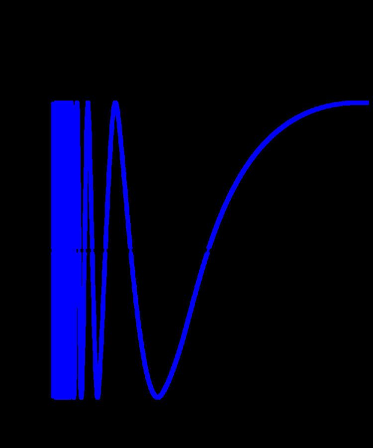
The function

is not of bounded variation on the interval [ 0 , 2 / π ]

While it is harder to see, the continuous function

is not of bounded variation on the interval [ 0 , 2 / π ] either.

At the same time, the function

is of bounded variation on the interval [ 0 , 2 / π ] . However, all three functions are of bounded variation on each interval [ a , b ] with a > 0 .

The Sobolev space W 1 , 1 ( Ω ) is a proper subset of B V ( Ω ) . In fact, for each u in W 1 , 1 ( Ω ) it is possible to choose a measure μ := ∇ u L (where L is the Lebesgue measure on Ω ) such that the equality

holds, since it is nothing more than the definition of weak derivative, and hence holds true. One can easily find an example of a BV function which is not W 1 , 1 : in dimension one, any step function with a non-trivial jump will do.

Mathematics

Functions of bounded variation have been studied in connection with the set of discontinuities of functions and differentiability of real functions, and the following results are well-known. If f is a real function of bounded variation on an interval [ a , b ] then

For real functions of several real variables

Physics and engineering

The ability of BV functions to deal with discontinuities has made their use widespread in the applied sciences: solutions of problems in mechanics, physics, chemical kinetics are very often representable by functions of bounded variation. The book (Hudjaev & Vol'pert 1985) details a very ample set of mathematical physics applications of BV functions. Also there is some modern application which deserves a brief description.