Arc length - Alchetron, The Free Social Encyclopedia

Determining the length of an irregular arc segment is also called rectification of a curve. Historically, many methods were used for specific curves. The advent of infinitesimal calculus led to a general formula that provides closed-form solutions in some cases.

General approach

A curve in the plane can be approximated by connecting a finite number of points on the curve using line segments to create a polygonal path. Since it is straightforward to calculate the length of each linear segment (using the Pythagorean theorem in Euclidean space, for example), the total length of the approximation can be found by summing the lengths of each linear segment; that approximation is known as the (cumulative) chordal distance.

If the curve is not already a polygonal path, using a progressively larger number of segments of smaller lengths will result in better approximations. The lengths of the successive approximations will not decrease and may keep increasing indefinitely, but for smooth curves they will tend to a finite limit as the lengths of the segments get arbitrarily small.

For some curves there is a smallest number L that is an upper bound on the length of any polygonal approximation. These curves are called rectifiable and the number L is defined as the arc length.

Definition for a smooth curve

Let f : [ a , b ] → R n be a continuously differentiable function. The length of the curve defined by f can be defined as the limit of the sum of line segment lengths for a regular partition of [ a , b ] as the number of segments approaches infinity. This means

L ( f ) = lim N → ∞ ∑ i = 1 N | f ( t i ) − f ( t i − 1 ) |

where t i = a + i ( b − a ) / N = a + i Δ t for i = 0 , 1 , … , N . This definition is equivalent to the standard definition of arc length as an integral:

The last equality above is true because the definition of the derivative as a limit implies that there is a positive real function δ ( ϵ ) of positive real ϵ such that Δ t < δ ( ϵ ) implies | | f ( t i ) − f ( t i − 1 ) Δ t | − | f ′ ( t i ) | | < ϵ . This means

∑ i = 1 N | f ( t i ) − f ( t i − 1 ) Δ t | Δ t − ∑ i = 1 N | f ′ ( t i ) | Δ t

has absolute value less than ϵ ( b − a ) for N > ( b − a ) / δ ( ϵ ) . This means that in the limit N → ∞ , the left term above equals the right term, which is just the Riemann integral of | f ′ ( t ) | on [ a , b ] . This definition of arc length shows that the length of a curve f : [ a , b ] → R n continuously differentiable on [ a , b ] is always finite. In other words, the curve is always rectifiable.

The definition of arc length of a smooth curve as the integral of the norm of the derivative is equivalent to the definition

L ( f ) = sup ∑ i = 1 N | f ( t i ) − f ( t i − 1 ) |

where the supremum is taken over all possible partitions a = t 0 < t 1 < ⋯ < t N − 1 < t N = b of [ a , b ] . This definition is also valid if f is merely continuous, not differentiable.

A curve can be parameterized in infinitely many ways. Let φ : [ a , b ] → [ c , d ] be any continuously differentiable bijection. Then g = f ∘ φ − 1 : [ c , d ] → R n is another continuously differentiable parameterization of the curve originally defined by f . The arc length of the curve is the same regardless of the parameterization used to define the curve:

Finding arc lengths by integrating

If a planar curve in R 2 is defined by the equation y = f ( x ) , where f is continuously differentiable, then it is simply a special case of a parametric equation where x = t and y = f ( t ) , the arc length is given by:

s = ∫ a b 1 + ( d y d x ) 2 d x .

Curves with closed-form solutions for arc length include the catenary, circle, cycloid, logarithmic spiral, parabola, semicubical parabola and straight line. The lack of a closed form solution for the arc length of an elliptic arc led to the development of the elliptic integrals.

Numerical integration

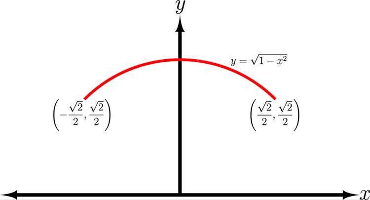
In most cases, including even simple curves, there are no closed-form solutions for arc length and numerical integration is necessary. Numerical integration of the arc length integral is usually very efficient. For example, consider the problem of finding the length of a quarter of the unit circle by numerically integrating the arc length integral. The upper half of the unit circle can be parameterized as y = 1 − x 2 . The interval x ∈ [ − 2 / 2 , 2 / 2 ] corresponds to a quarter of the circle. Since d y / d x = − x / 1 − x 2 and 1 + ( d y / d x ) 2 = 1 / ( 1 − x 2 ) , the length of a quarter of the unit circle is

∫ − 2 / 2 2 / 2 1 1 − x 2 d x .

The 15-point Gauss-Kronrod rule estimate for this integral of 1.570796326808177 differs from the true length of π / 2 by 1.3e-11 and the 16-point Gaussian quadrature rule estimate of 1.570796326794727 differs from the true length by only 1.7e-13. This means it is possible to evaluate this integral to almost machine precision with only 16 integrand evaluations.

Curve on a surface

Let x ( u , v ) be a surface mapping and let C ( t ) = ( u ( t ) , v ( t ) ) be a curve on this surface. The integrand of the arc length integral is | ( x ∘ C ) ′ ( t ) | . Evaluating the derivative requires the chain rule for vector fields:

D ( x ∘ C ) = ( x u x v ) ( u ′ v ′ ) = x u u ′ + x v v ′ .

The squared norm of this vector is ( x u u ′ + x v v ′ ) ⋅ ( x u u ′ + x v v ′ ) = g 11 ( u ′ ) 2 + 2 g 12 u ′ v ′ + g 22 ( v ′ ) 2 (where g i j is the first fundamental form coefficient), so the integrand of the arc length integral can be written as g a b ( u a ) ′ ( u b ) ′ (where u 1 = u and u 2 = v ).

Other coordinate systems

Let C ( t ) = ( r ( t ) , θ ( t ) ) be a curve expressed in polar coordinates. The mapping that transforms from polar coordinates to rectangular coordinates is

x ( r , θ ) = ( r cos ⁡ θ , r sin ⁡ θ ) .

The integrand of the arc length integral is | ( x ∘ C ) ′ ( t ) | . The chain rule for vector fields shows that D ( x ∘ C ) = x r r ′ + x θ θ ′ . So the squared integrand of the arc length integral is

( x r ⋅ x r ) ( r ′ ) 2 + 2 ( x r ⋅ x θ ) r ′ θ ′ + ( x θ ⋅ x θ ) ( θ ′ ) 2 = ( r ′ ) 2 + r 2 ( θ ′ ) 2 .

So for a curve expressed in polar coordinates, the arc length is

∫ t 1 t 2 ( d r d t ) 2 + r 2 ( d θ d t ) 2 d t = ∫ θ ( t 1 ) θ ( t 2 ) ( d r d θ ) 2 + r 2 d θ .

Now let C ( t ) = ( r ( t ) , θ ( t ) , ϕ ( t ) ) be a curve expressed in spherical coordinates where θ is the polar angle measured from the positive z -axis and ϕ is the azimuthal angle. The mapping that transforms from spherical coordinates to rectangular coordinates is

x ( r , θ , ϕ ) = ( r sin ⁡ θ cos ⁡ ϕ , r sin ⁡ θ sin ⁡ ϕ , r cos ⁡ θ ) .

Using the chain rule again shows that D ( x ∘ C ) = x r r ′ + x θ θ ′ + x ϕ ϕ ′ . All dot products x i ⋅ x j where i and j differ are zero, so the squared norm of this vector is

( x r ⋅ x r ) ( r ′ 2 ) + ( x θ ⋅ x θ ) ( θ ′ ) 2 + ( x ϕ ⋅ x ϕ ) ( ϕ ′ ) 2 = ( r ′ ) 2 + r 2 ( θ ′ ) 2 + r 2 sin 2 ⁡ θ ( ϕ ′ ) 2 .

So for a curve expressed in spherical coordinates, the arc length is

∫ t 1 t 2 ( d r d t ) 2 + r 2 ( d θ d t ) 2 + r 2 sin 2 ⁡ θ ( d ϕ d t ) 2 d t .

A very similar calculation shows that the arc length of a curve expressed in cylindrical coordinates is

∫ t 1 t 2 ( d r d t ) 2 + r 2 ( d θ d t ) 2 + ( d z d t ) 2 d t .

Arcs of circles

Arc lengths are denoted by s, since the Latin word for length (or size) is spatium.

In the following lines, r represents the radius of a circle, d is its diameter, C is its circumference, s is the length of an arc of the circle, and θ is the angle which the arc subtends at the centre of the circle. The distances r , d , C , and s are expressed in the same units.

C = 2 π r , which is the same as C = π d . This equation is a definition of π .

If the arc is a semicircle, then s = π r .

For an arbitrary circular arc:

If θ is in radians then s = r θ . This is a definition of the radian.

If θ is in degrees, then s = π r θ 180 , which is the same as s = C θ 360 .

If θ is in grads (100 grads, or grades, or gradians are one right-angle), then s = π r θ 200 , which is the same as s = C θ 400 .

If θ is in turns (one turn is a complete rotation, or 360°, or 400 grads, or 2 π radians), then s = C θ .

Arcs of great circles on the Earth

Two units of length, the nautical mile and the metre (or kilometre), were originally defined so the lengths of arcs of great circles on the Earth's surface would be simply numerically related to the angles they subtend at its centre. The simple equation s = θ applies in the following circumstances:

if s is in nautical miles, and θ is in arcminutes ( ¹⁄₆₀ degree), or

if s is in kilometres, and θ is in centigrades ( ¹⁄₁₀₀ grad).

The lengths of the distance units were chosen to make the circumference of the Earth equal 40,000 kilometres, or 21,600 nautical miles. These are the numbers of the corresponding angle units in one complete turn.

These definitions of the metre and nautical mile have been superseded by more precise ones, but the original definitions are still accurate enough for conceptual purposes, and for some calculations. For example, they imply that one kilometre is exactly 0.54 nautical miles. Using official modern definitions, one nautical mile is exactly 1.852 kilometres, which implies that 1 kilometre ≈ 0.53995680 nautical miles. This modern ratio differs from the one calculated from the original definitions by less than one part in ten thousand.

Antiquity

For much of the history of mathematics, even the greatest thinkers considered it impossible to compute the length of an irregular arc. Although Archimedes had pioneered a way of finding the area beneath a curve with his "method of exhaustion", few believed it was even possible for curves to have definite lengths, as do straight lines. The first ground was broken in this field, as it often has been in calculus, by approximation. People began to inscribe polygons within the curves and compute the length of the sides for a somewhat accurate measurement of the length. By using more segments, and by decreasing the length of each segment, they were able to obtain a more and more accurate approximation. In particular, by inscribing a polygon of many sides in a circle, they were able to find approximate values of π.

17th century

In the 17th century, the method of exhaustion led to the rectification by geometrical methods of several transcendental curves: the logarithmic spiral by Evangelista Torricelli in 1645 (some sources say John Wallis in the 1650s), the cycloid by Christopher Wren in 1658, and the catenary by Gottfried Leibniz in 1691.

In 1659, Wallis credited William Neile's discovery of the first rectification of a nontrivial algebraic curve, the semicubical parabola.

Integral form

Before the full formal development of calculus, the basis for the modern integral form for arc length was independently discovered by Hendrik van Heuraet and Pierre de Fermat.

In 1659 van Heuraet published a construction showing that the problem of determining arc length could be transformed into the problem of determining the area under a curve (i.e., an integral). As an example of his method, he determined the arc length of a semicubical parabola, which required finding the area under a parabola. In 1660, Fermat published a more general theory containing the same result in his De linearum curvarum cum lineis rectis comparatione dissertatio geometrica (Geometric dissertation on curved lines in comparison with straight lines).

Building on his previous work with tangents, Fermat used the curve

y = x 3 / 2

whose tangent at x = a had a slope of

3 2 a 1 / 2

so the tangent line would have the equation

y = 3 2 a 1 / 2 ( x − a ) + f ( a ) .

Next, he increased a by a small amount to a + ε, making segment AC a relatively good approximation for the length of the curve from A to D. To find the length of the segment AC, he used the Pythagorean theorem:

A C 2 = A B 2 + B C 2 = ε 2 + 9 4 a ε 2 = ε 2 ( 1 + 9 4 a )

which, when solved, yields

A C = ε 1 + 9 4 a .

In order to approximate the length, Fermat would sum up a sequence of short segments.

Curves with infinite length

As mentioned above, some curves are non-rectifiable. That is, there is no upper bound on the lengths of polygonal approximations; the length can be made arbitrarily large. Informally, such curves are said to have infinite length. There are continuous curves on which every arc (other than a single-point arc) has infinite length. An example of such a curve is the Koch curve. Another example of a curve with infinite length is the graph of the function defined by f(x) = x sin(1/x) for any open set with 0 as one of its delimiters and f(0) = 0. Sometimes the Hausdorff dimension and Hausdorff measure are used to quantify the size of such curves.

Generalization to (pseudo-)Riemannian manifolds

Let M be a (pseudo-)Riemannian manifold, γ : [ 0 , 1 ] → M a curve in M and g the (pseudo-) metric tensor.

The length of γ is defined to be

ℓ ( γ ) = ∫ 0 1 ± g ( γ ′ ( t ) , γ ′ ( t ) ) d t ,

where γ ′ ( t ) ∈ T γ ( t ) M is the tangent vector of γ at t . The sign in the square root is chosen once for a given curve, to ensure that the square root is a real number. The positive sign is chosen for spacelike curves; in a pseudo-Riemannian manifold, the negative sign may be chosen for timelike curves . Thus the length of a curve in a non-negative real number. Usually no curves are considered which are partly spacelike and partly timelike.

In theory of relativity, arc length of timelike curves (world lines) is the proper time elapsed along the world line, and arc length of a spacelike curve the proper distance along the curve.

References

Arc length Wikipedia

(Text) CC BY-SA

Contents