
 | ||
In statistics, the variance function is a smooth function which depicts the variance of a random quantity as a function of its mean. The variance function plays a large role in many settings of statistical modelling. It is a main ingredient in the generalized linear model framework and a tool used in non-parametric regression, semiparametric regression and functional data analysis. In parametric modeling, variance functions take on a parametric form and explicitly describe the relationship between the variance and the mean of a random quantity. In a non-parametric setting, the variance function is assumed to be a smooth function.
Contents
Intuition
In a regression model setting, the goal is to establish whether or a not a relationship exists between a response variable and a set of predictor variables. Further, if a relationship does exist, the goal is then to be able to describe this relationship as best as possible. A main assumption in linear regression is constant variance or (homoscedasticity), meaning that different response variables have the same variance in their errors, at every predictor level. This assumption works well when the response variable and the predictor variable are jointly Normal, see Normal distribution. As we will see later, the variance function in the Normal setting, is constant, however, we must find a way to quantify heteroscedasticity (non-constant variance) in the absence of joint Normality.
When it is likely that the response follows a distribution that is a member of the exponential family, a generalized linear model may be more appropriate to use, and moreover, when we wish not to force a parametric model onto our data, a non-parametric regression approach can be useful. The importance of being able to model the variance as a function of the mean lies in improved inference (in a parametric setting), and estimation of the regression function in general, for any setting.
Variance functions play a very important role in parameter estimation and inference. In general, maximum likelihood estimation requires that a likelihood function be defined. This requirement then implies that one must first specify the distribution of the response variables observed. However, to define a quasi-likelihood, one need only specify a relationship between the mean and the variance of the observations to then be able to use the quasi-likelihood function for estimation. Quasi-likelihood estimation is particularly useful when there is overdispersion. Overdispersion occurs when there is more variability in the data than there should otherwise be expected according to the assumed distribution of the data.
In summary, to ensure efficient inference of the regression parameters and the regression function, the heteroscedasticity must be accounted for. Variance functions quantify the relationship between the variance and the mean of the observed data and hence play a significant role in regression estimation and inference.
Types of variance functions
The variance function and its applications come up in many areas of statistical analysis. A very important use of this function is in the framework of generalized linear models and non-parametric regression.
Generalized linear model
When a member of the exponential family has been specified, the variance function can easily be derived. The general form of the variance function is presented under the exponential family context, as well as specific forms for Normal, Bernoulli, Poisson, and Gamma. In addition, we describe the applications and use of variance functions in maximum likelihood estimation and quasi-likelihood estimation.
Derivation
The generalized linear model (GLM), is a generalization of ordinary regression analysis that extends to any member of the exponential family. It is particularly useful when the response variable is categorical, binary or subject to a constraint (e.g. only positive responses make sense). A quick summary of the components of a GLM are summarized on this page, but for more details and information see the page on generalized linear models.
A GLM consists of three main ingredients:
1. Random Component: a distribution of y from the exponential family,First it is important to derive a couple key properties of the exponential family.
Any random variable
with loglikelihood,
Here,
These identities lead to simple calculations of the expected value and variance of any random variable
Expected value of Y: Taking the first derivative with respect to
Then taking the expected value and setting it equal to zero leads to,
Variance of Y: To compute the variance we use the second Bartlett identity,
We have now a relationship between
Note that because
Example – normal
The Normal distribution is a special case where the variance function is a constant. Let
where
To calculate the variance function
Therefore the variance function is constant.
Example – Bernoulli
Let
This give us
Example – Poisson
Let
This give us
Here we see the central property of Poisson data, that the variance is equal to the mean.
Example – Gamma
The Gamma distribution and density function can be expressed under different parametrizations. We will use the form of the gamma with parameters
Then in exponential family form we have
And we have
Application – weighted least squares
A very important application of the variance function is its use in parameter estimation and inference when the response variable is of the required exponential family form as well as in some cases when it is not (which we will discuss in quasi-likelihood). Weighted least squares (WLS) is a special case of generalized least squares. Each term in the WLS criterion includes a weight that determines that the influence each observation has on the final parameter estimates. As in regular least squares, the goal is to estimate the unknown parameters in the regression function by finding values for parameter estimates that minimize the sum of the squared deviations between the observed responses and the functional portion of the model.
While WLS assumes independence of observations it does not assume equal variance and is therefore a solution for parameter estimation in the presence of heteroscedasticity. The Gauss–Markov theorem and Aitken demonstrate that the best linear unbiased estimator (BLUE), the unbiased estimator with minimum variance, has each weight equal to the reciprocal of the variance of the measurement.
In the GLM framework, our goal is to estimate parameters
where
Also, important to note is that when the weight matrix is of the form described here, minimizing the expression
The matrix W falls right out of the estimating equations for estimation of
Looking at a single observation we have,
This gives us
The Hessian matrix is determined in a similar manner and can be shown to be,
Noticing that the Fisher Information (FI),
Application – quasi-likelihood
Because most features of GLMs only depend on the first two moments of the distribution, rather than then entire distribution, the quasi-likelihood can be developed by just specifying a link function and a variance function. That is, we need to specify
– Link function:With a specified variance function and link function we can develop, as alternatives to the log-likelihood function, the score function, and the Fisher information, a quasi-likelihood, a quasi-score, and the quasi-information. This allows for full inference of
Quasi-likelihood (QL)
Though called a quasi-likelihood, this is in fact a quasi-log-likelihood. The QL for one observation is
And therefore the QL for all n observations is
From the QL we have the quasi-score
Quasi-score (QS)
Recall the score function, U, for data with log-likelihood
We obtain the quasi-score in an identical manner,
Noting that, for one observation the score is
The first two Bartlett equations are satisfied for the quasi-score, namely
and
In addition, the quasi-score is linear in y.
Ultimately the goal is to find information about the parameters of interest
Quasi-information (QI)
The quasi-information, is similar to the Fisher information,
QL,QS,QI as functions of
The QL, QS and QI all provide the building blocks for inference about the parameters of interest and therefore it is important to express the QL, QS and QI all as functions of
Recalling again that
Quasi-likelihood in
The QS as a function of
Where,
The quasi-information matrix in
Obtaining the score function and the information of
Non-parametric regression analysis
Non-parametric estimation of the variance function and its importance, has been discussed widely in the literature In non-parametric regression analysis, the goal is to express the expected value of your response variable(y) as a function of your predictors (X). That is we are looking to estimate a mean function,
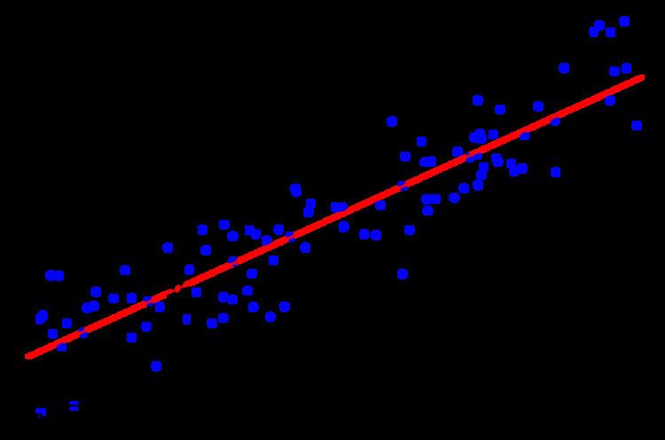
An example is detailed in the pictures to the left. The goal of the project was to determine (among other things) whether or not the predictor, number of years in the major leagues (baseball,) had an effect on the response, salary, a player made. An initial scatter plot of the data indicates that there is heteroscedasticity in the data as the variance is not constant at each level of the predictor. Because we can visually detect the non-constant variance, it useful now to plot