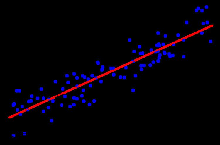
 | ||
The method of iteratively reweighted least squares (IRLS) is used to solve certain optimization problems with objective functions of the form:
Contents
by an iterative method in which each step involves solving a weighted least squares problem of the form:
IRLS is used to find the maximum likelihood estimates of a generalized linear model, and in robust regression to find an M-estimator, as a way of mitigating the influence of outliers in an otherwise normally-distributed data set. For example, by minimizing the least absolute error rather than the least square error.
Although not a linear regression problem, Weiszfeld's algorithm for approximating the geometric median can also be viewed as a special case of iteratively reweighted least squares, in which the objective function is the sum of distances of the estimator from the samples.
One of the advantages of IRLS over linear programming and convex programming is that it can be used with Gauss–Newton and Levenberg–Marquardt numerical algorithms.
L1 minimization for sparse recovery
IRLS can be used for ℓ1 minimization and smoothed ℓp minimization, p < 1, in the compressed sensing problems. It has been proved that the algorithm has a linear rate of convergence for ℓ1 norm and superlinear for ℓt with t < 1, under the restricted isometry property, which is generally a sufficient condition for sparse solutions. However in most practical situations, the restricted isometry property is not satisfied.
Lp norm linear regression
To find the parameters β = (β1, …,βk)T which minimize the Lp norm for the linear regression problem,
the IRLS algorithm at step t + 1 involves solving the weighted linear least squares problem:
where W(t) is the diagonal matrix of weights, usually with all elements set initially to:
and updated after each iteration to:
In the case p = 1, this corresponds to least absolute deviation regression (in this case, the problem would be better approached by use of linear programming methods, so the result would be exact) and the formula is:
To avoid dividing by zero, regularization must be done, so in practice the formula is:
where
