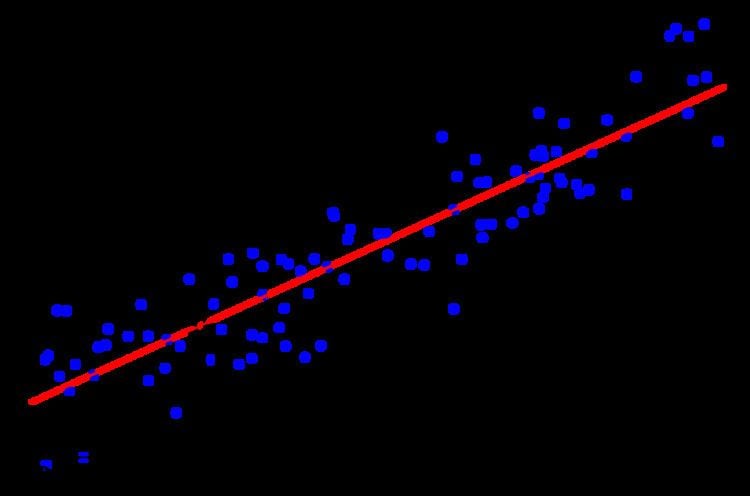
Gauss–Markov theorem - Alchetron, The Free Social Encyclopedia

In statistics, the Gauss–Markov theorem, named after Carl Friedrich Gauss and Andrey Markov, states that in a linear regression model in which the errors have expectation zero and are uncorrelated and have equal variances, the best linear unbiased estimator (BLUE) of the coefficients is given by the ordinary least squares (OLS) estimator, provided it exists. Here "best" means giving the lowest variance of the estimate, as compared to other unbiased, linear estimators. The errors do not need to be normal, nor do they need to be independent and identically distributed (only uncorrelated with mean zero and homoscedastic with finite variance). The requirement that the estimator be unbiased cannot be dropped, since biased estimators exist with lower variance. See, for example, the James–Stein estimator (which also drops linearity) or ridge regression.

Statement

Suppose we have in matrix notation,

y _ = X β _ + ε _ , ( y _ , ε _ ∈ R n , β _ ∈ R K and X ∈ R n × K )

expanding to,

y i = ∑ j = 1 K β j X i j + ε i ∀ i = 1 , 2 , … , n

where β j are non-random but unobservable parameters, X i j are non-random and observable (called the "explanatory variables"), ε i are random, and so y i are random. The random variables ε i are called the "disturbance", "noise" or simply "error" (will be contrasted with "residual" later in the article; see errors and residuals in statistics). Note that to include a constant in the model above, one can choose to introduce the constant as a variable β K + 1 with a newly introduced last column of X being unity i.e., X i ( K + 1 ) = 1 for all i .

The Gauss–Markov assumptions concern the set of error random variables, ε i :

They have mean zero: E [ ε i ] = 0.

They are homoscedastic, that is all have the same finite variance: Var ( ε i ) = σ 2 < ∞ , and

Distinct error terms are uncorrelated: Cov ( ε i , ε j ) = 0 , ∀ i ≠ j .

A linear estimator of β j is a linear combination

β ^ j = c 1 j y 1 + ⋯ + c n j y n

in which the coefficients c i j are not allowed to depend on the underlying coefficients β j , since those are not observable, but are allowed to depend on the values X i j , since these data are observable. (The dependence of the coefficients on each X i j is typically nonlinear; the estimator is linear in each y i and hence in each random ε , which is why this is "linear" regression.) The estimator is said to be unbiased if and only if

E [ β ^ j ] = β j

regardless of the values of X i j . Now, let ∑ j = 1 K λ j β j be some linear combination of the coefficients. Then the mean squared error of the corresponding estimation is

E [ ( ∑ j = 1 K λ j ( β ^ j − β j ) ) 2 ] ,

in other words it is the expectation of the square of the weighted sum (across parameters) of the differences between the estimators and the corresponding parameters to be estimated. (Since we are considering the case in which all the parameter estimates are unbiased, this mean squared error is the same as the variance of the linear combination.) The best linear unbiased estimator (BLUE) of the vector β of parameters β j is one with the smallest mean squared error for every vector λ of linear combination parameters. This is equivalent to the condition that

Var ( β ~ ) − Var ( β ^ )

is a positive semi-definite matrix for every other linear unbiased estimator β ~ .

The ordinary least squares estimator (OLS) is the function

β ^ = ( X ′ X ) − 1 X ′ y

of y and X (where X ′ denotes the transpose of X ) that minimizes the sum of squares of residuals (misprediction amounts):

∑ i = 1 n ( y i − y ^ i ) 2 = ∑ i = 1 n ( y i − ∑ j = 1 K β ^ j X i j ) 2 .

The theorem now states that the OLS estimator is a BLUE. The main idea of the proof is that the least-squares estimator is uncorrelated with every linear unbiased estimator of zero, i.e., with every linear combination a 1 y 1 + ⋯ + a n y n whose coefficients do not depend upon the unobservable β but whose expected value is always zero.

Proof

Let β ~ = C y be another linear estimator of β with C = ( X ′ X ) − 1 X ′ + D where D is a K × n non-zero matrix. As we're restricting to unbiased estimators, minimum mean squared error implies minimum variance. The goal is therefore to show that such an estimator has a variance no smaller than that of β ^ , the OLS estimator. We calculate:

E [ β ~ ] = E [ C y ] = E [ ( ( X ′ X ) − 1 X ′ + D ) ( X β + ε ) ] = ( ( X ′ X ) − 1 X ′ + D ) X β + ( ( X ′ X ) − 1 X ′ + D ) E [ ε ] = ( ( X ′ X ) − 1 X ′ + D ) X β E [ ε ] = 0 = ( X ′ X ) − 1 X ′ X β + D X β = ( I K + D X ) β .

Therefore, β ~ is unbiased if and only if D X = 0 . Then:

Var ( β ~ ) = Var ( C y ) = C Var ( y ) C ′ = σ 2 C C ′ = σ 2 ( ( X ′ X ) − 1 X ′ + D ) ( X ( X ′ X ) − 1 + D ′ ) = σ 2 ( ( X ′ X ) − 1 X ′ X ( X ′ X ) − 1 + ( X ′ X ) − 1 X ′ D ′ + D X ( X ′ X ) − 1 + D D ′ ) = σ 2 ( X ′ X ) − 1 + σ 2 ( X ′ X ) − 1 ( D X ) ′ + σ 2 D X ( X ′ X ) − 1 + σ 2 D D ′ = σ 2 ( X ′ X ) − 1 + σ 2 D D ′ D X = 0 = Var ( β ^ ) + σ 2 D D ′ σ 2 ( X ′ X ) − 1 = Var ( β ^ )

Since DD' is a positive semidefinite matrix, Var ( β ~ ) exceeds Var ( β ^ ) by a positive semidefinite matrix.

Remarks on the proof

As it has been stated before, the condition of Var ( β ~ ) − Var ( β ^ ) is equivalent to the property that the best linear unbiased estimator of l t β is l t β ^ (best in the sense that it has minimum variance). To see this, let l t β ~ another linear unbiased estimator of l t β .

Var ( l t β ~ ) = l t Var ( β ~ ) l = σ 2 l t ( X ′ X ) − 1 l + l t D D t l = Var ( l t β ^ ) + ( D t l ) t ( D t l ) σ 2 l t ( X ′ X ) − 1 l = Var ( l t β ^ ) = Var ( l t β ^ ) + ∥ D t l ∥ ⩾ Var ( l t β ^ )

Moreover equality holds if and only if D t l = 0 . We calculate

l t β ~ = l t ( ( ( X ′ X ) − 1 X ′ + D ) Y ) from above = l t ( X ′ X ) − 1 X ′ Y + l t D Y = l t β ^ + ( D t l ) t Y = l t β ^ D t l = 0

This proves that the equality holds if and only if l t β ~ = l t β ^ which gives the uniqueness of the OLS estimator as a BLUE.

Generalized least squares estimator

The generalized least squares (GLS), developed by Aitken, extends the Gauss–Markov theorem to the case where the error vector has a non-scalar covariance matrix. The Aitken estimator is also a BLUE.

Gauss–Markov theorem as stated in econometrics

In most treatments of OLS, the regressors in the design matrix X are assumed to be fixed in repeated samples. This assumption is considered inappropriate for a predominantly nonexperimental science like econometrics. Instead, the assumptions of the Gauss–Markov theorem are stated conditional on X .

Linearity

The dependent variable is assumed to be a linear function of the variables specified in the model. The specification must be linear in its parameters. This does not mean that there must be a linear relationship between the independent and dependent variables. The independent variables can take non-linear forms as long as the parameters are linear. The equation y = β 0 + β 1 x 2 , qualifies as linear while y = β 0 + β 1 2 x can be transformed to be linear by replacing β 1 2 by another parameter, say γ . An equation with a parameter dependent on an independent variable does not qualify as linear, for example y = β 0 + β 1 ( x ) ⋅ x , where β 1 ( x ) is a function of x .

Data transformations are often used to convert an equation into a linear form. For example, the Cobb–Douglas function—often used in economics—is nonlinear:

Y = A L α K 1 − α e ε

But it can be expressed in linear form by taking the natural logarithm of both sides:

ln ⁡ Y = ln ⁡ A + α ln ⁡ L + ( 1 − α ) ln ⁡ K + ε = β 0 + β 1 ln ⁡ L + β 2 ln ⁡ K + ε

This assumption also covers specification issues: assuming that the proper functional form has been selected and there are no omitted variables.

Strict exogeneity

For all n observations, the expectation—conditional on the regressors—of the error term is zero:

E ⁡ [ ε i | X ] = E ⁡ [ ε i | x 1 , … , x n ] = 0.

where x i = [ x i 1 x i 2 … x i k ] T is the data vector of regressors for the ith observation, and consequently X = [ x 1 T x 2 T … x n T ] T is the data matrix or design matrix.

Geometrically, this assumptions implies that x i and ε i are orthogonal to each other, so that their inner product (i.e., their cross moment) is zero.

E ⁡ [ x j ⋅ ε i ] = [ E ⁡ [ x j 1 ⋅ ε i ] E ⁡ [ x j 2 ⋅ ε i ] ⋮ E ⁡ [ x j k ⋅ ε i ] ] = 0 for all i , j ∈ n

This assumption is violated if the explanatory variables are stochastic, for instance when they are measured with error, or are endogenous. Endogeneity can be the result of simultaneity, where causality flows back and forth between both the dependent and independent variable. Instrumental variable techniques are commonly used to address this problem.

Full rank

The sample data matrix X must be non-singular, i.e. it must have full rank.

rank ⁡ ( X ) = k

Otherwise X is not invertible and the OLS estimator cannot be computed.

A violation of this assumption is perfect multicollinearity, i.e. some explanatory variables are linearly dependent. One scenario in which this will occur is called "dummy variable trap," when a base dummy variable is not omitted resulting in perfect correlation between the dummy variables and the constant term.

Multicollinearity (as long as it is not "perfect") can be present resulting in a less efficient, but still unbiased estimate. The estimates will be less precise and highly sensitive to particular sets of data. Multicollinearity can be detected from condition number or the variance inflation factor, among other tests.

Spherical errors

The outer product of the error vector must be spherical.

E ⁡ [ ε ε T | X ] = Var ⁡ [ ε | X ] = [ σ 2 0 … 0 0 σ 2 … 0 ⋮ ⋮ ⋱ ⋮ 0 0 … σ 2 ] = σ 2 I with σ 2 > 0

This implies the error term has uniform variance (homoscedasticity) and no serial dependence. If this assumption is violated, OLS is still unbiased, but inefficient. The term "spherical errors" will describe the multivariate normal distribution: if Var ⁡ [ ε | X ] = σ 2 I in the multivariate normal density, then the equation f(x)=c is the formula for a “ball” centered at μ with radius σ in n-dimensional space.

Heteroskedasticity occurs when the amount of error is correlated with an independent variable. For example, in a regression on food expenditure and income, the error is correlated with income. Low income people generally spend a similar amount on food, while high income people may spend a very large amount or as little as low income people spend. Heteroskedacity can also be caused by changes in measurement practices. For example, as statistical offices improve their data, measurement error decreases, so the error term declines over time.

This assumption is violated when there is autocorrelation. Autocorrelation can be visualized on a data plot when a given observation is more likely to lie above a fitted line if adjacent observations also lie above the fitted regression line. Autocorrelation is common in time series data where a data series may experience "inertia." If a dependent variable takes a while to fully absorb a shock. Spatial autocorrelation can also occur geographic areas are likely to have similar errors. Autocorrelation may be the result of misspecification such as choosing the wrong functional form. In these cases, correcting the specification is one possible way to deal with autocorrelation.

In the presence of non-spherical errors, the generalized least squares estimator can be shown to be BLUE.

References

Gauss–Markov theorem Wikipedia

(Text) CC BY-SA