Leibniz integral rule

General form: Differentiation under the integral sign

Theorem. Let f(x, t) be a function such that both f(x, t) and its partial derivative f_x(x, t) are continuous in t and x in some region of the (x, t)-plane, including a(x) ≤ t ≤ b(x), x₀ ≤ x ≤ x₁. Also suppose that the functions a(x) and b(x) are both continuous and both have continuous derivatives for x₀ ≤ x ≤ x₁. Then for x₀ ≤ x ≤ x₁: d d x ( ∫ a ( x ) b ( x ) f ( x , t ) d t ) = f ( x , b ( x ) ) ⋅ d d x b ( x ) − f ( x , a ( x ) ) ⋅ d d x a ( x ) + ∫ a ( x ) b ( x ) ∂ ∂ x f ( x , t ) d t .

This formula is the general form of the Leibniz integral rule and can be derived using the fundamental theorem of calculus. The (first) fundamental theorem of calculus is just a particular case of the above formula, for a(x) = a, a constant, b(x) = x and f(x, t) = f(t).

If both upper and lower limits are taken as constants, then the formula takes the shape of an operator equation:

I_tD_x = D_xI_t,

where D_x is the partial derivative with respect to x and I_t is the integral operator with respect to t over a fixed interval. That is, it is related to the symmetry of second derivatives, but involving integrals as well as derivatives. This case is also known as the Leibniz integral rule.

The following three basic theorems on the interchange of limits are essentially equivalent:

the interchange of a derivative and an integral (differentiation under the integral sign; i.e., Leibniz integral rule)

the change of order of partial derivatives

the change of order of integration (integration under the integral sign; i.e., Fubini's theorem)

Three-dimensional, time-dependent case

A Leibniz integral rule for two dimensions is:

d d t ∬ Σ ( t ) F ( r , t ) ⋅ d A = ∬ Σ ( t ) ( F t ( r , t ) + [ ∇ ⋅ F ( r , t ) ] v ) ⋅ d A − ∮ ∂ Σ ( t ) [ v × F ( r , t ) ] ⋅ d s

where:

Higher dimensions

The Leibniz integral rule can be extended to multidimensional integrals. In two and three dimensions, this rule is better known from the field of fluid dynamics as the Reynolds transport theorem:

d d t ∫ D ( t ) F ( x → , t ) d V = ∫ D ( t ) ∂ ∂ t F ( x → , t ) d V + ∫ ∂ D ( t ) F ( x → , t ) v → b ⋅ d Σ

where F ( x → , t ) is a scalar function, D(t) and ∂D(t) denote a time-varying connected region of R³ and its boundary, respectively, v → b is the Eulerian velocity of the boundary (see Lagrangian and Eulerian coordinates) and dΣ = n dS is the unit normal component of the surface element.

The general statement of the Leibniz integral rule requires concepts from differential geometry, specifically differential forms, exterior derivatives, wedge products and interior products. With those tools, the Leibniz integral rule in p-dimensions is:

d d t ∫ Ω ( t ) ω = ∫ Ω ( t ) i v → ( d x ω ) + ∫ ∂ Ω ( t ) i v → ω + ∫ Ω ( t ) ω ˙ ,

where Ω(t) is a time-varying domain of integration, ω is a p-form, v → is the vector field of the velocity, v → = ∂ x → ∂ t , i denotes the interior product, d_xω is the exterior derivative of ω with respect to the space variables only and ω ˙ is the time-derivative of ω.

Measure theory statement

Let X be an open subset of R , and Ω be a measure space. Suppose f : X × Ω → R satisfies the following conditions:

Then for all x ∈ X

Proof of basic form

Let:

u ( x ) = ∫ y 0 y 1 f ( x , y ) d y ( 1 )

So that, using difference quotients

u ′ ( x ) = lim h → 0 u ( x + h ) − u ( x ) h ( 2 )

Substitute equation (1) into equation (2), combine the integrals (since the difference of two integrals equals the integral of the difference) and use the fact that 1/h is a constant:

u ′ ( x ) = lim h → 0 ∫ y 0 y 1 f ( x + h , y ) d y − ∫ y 0 y 1 f ( x , y ) d y h = lim h → 0 ∫ y 0 y 1 ( f ( x + h , y ) − f ( x , y ) ) d y h = lim h → 0 ∫ y 0 y 1 f ( x + h , y ) − f ( x , y ) h d y

Provided that the limit can be passed under the integral sign, we obtain

u ′ ( x ) = ∫ y 0 y 1 f x ( x , y ) d y

We claim that the passage of the limit under the integral sign is valid. Indeed, the bounded convergence theorem (a corollary of the dominated convergence theorem) of real analysis states that if a sequence of functions on a set of finite measure is uniformly bounded and converges pointwise, then passage of the limit under the integral is valid. To complete the proof, we show that these hypotheses are satisfied by the family of difference quotients

f n ( y ) = f ( x + 1 n , y ) − f ( x , y ) 1 n .

Continuity of f_x(x, y) and compactness implies that f_x(x, y) is uniformly bounded. Uniform boundedness of the difference quotients follows from uniform boundedness of f_x(x, y) and the mean value theorem, since for all y and n, there exists z in the interval [x, x + 1/n] such that

f x ( z , y ) = f ( x + 1 n , y ) − f ( x , y ) 1 n .

The difference quotients converge pointwise to f_x(x, y) since f_x(x, y) exists. This completes the proof.

For a simpler proof using Fubini's theorem, see the references.

Variable limits form

For a monovariant function g:

d d x ( ∫ f 1 ( x ) f 2 ( x ) g ( t ) d t ) = g [ f 2 ( x ) ] f 2 ′ ( x ) − g [ f 1 ( x ) ] f 1 ′ ( x )

This follows from the chain rule.

General form with variable limits

Now, set

φ ( α ) = ∫ a b f ( x , α ) d x ,

where a and b are functions of α that exhibit increments Δa and Δb, respectively, when α is increased by Δα. Then,

Δ φ = φ ( α + Δ α ) − φ ( α ) = ∫ a + Δ a b + Δ b f ( x , α + Δ α ) d x − ∫ a b f ( x , α ) d x = ∫ a + Δ a a f ( x , α + Δ α ) d x + ∫ a b f ( x , α + Δ α ) d x + ∫ b b + Δ b f ( x , α + Δ α ) d x − ∫ a b f ( x , α ) d x = − ∫ a a + Δ a f ( x , α + Δ α ) d x + ∫ a b [ f ( x , α + Δ α ) − f ( x , α ) ] d x + ∫ b b + Δ b f ( x , α + Δ α ) d x

A form of the mean value theorem, ∫ a b f ( x ) d x = ( b − a ) f ( ξ ) , where a < ξ < b, may be applied to the first and last integrals of the formula for Δφ above, resulting in

Δ φ = − Δ a f ( ξ 1 , α + Δ α ) + ∫ a b [ f ( x , α + Δ α ) − f ( x , α ) ] d x + Δ b f ( ξ 2 , α + Δ α )

Dividing by Δα, and letting Δα → 0, and noticing ξ₁ → a and ξ₂ → b and using the result

lim Δ α → 0 ∫ a b f ( x , α + Δ α ) − f ( x , α ) Δ α d x = ∫ a b ∂ ∂ α f ( x , α ) d x

yields the general form of the Leibniz integral rule below:

d φ d α = ∫ a b ∂ ∂ α f ( x , α ) d x + f ( b , α ) d b d α − f ( a , α ) d a d α

Three-dimensional, time-dependent form

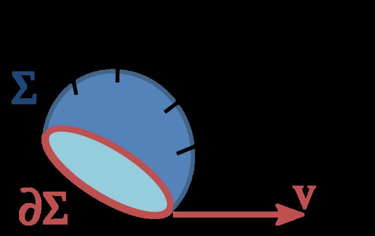
At time t the surface Σ in Figure 1 contains a set of points arranged about a centroid C ( t ) and function F ( r , t ) can be written as

F ( C ( t ) , r − C ( t ) , t ) = F ( C ( t ) + I , t ) ,

with I independent of time. Variables are shifted to a new frame of reference attached to the moving surface, with origin at C ( t ) . For a rigidly translating surface, the limits of integration are then independent of time, so:

d d t ( ∬ Σ ( t ) d A r ⋅ F ( r , t ) ) = ∬ Σ d A I ⋅ d d t F ( C ( t ) + I , t )

where the limits of integration confining the integral to the region Σ no longer are time dependent so differentiation passes through the integration to act on the integrand only:

d d t F ( C ( t ) + I , t ) = F t ( C ( t ) + I , t ) + v ⋅ ∇ F ( C ( t ) + I , t ) = F t ( r , t ) + v ⋅ ∇ F ( r , t )

with the velocity of motion of the surface defined by:

v = d d t C ( t )

This equation expresses the material derivative of the field, that is, the derivative with respect to a coordinate system attached to the moving surface. Having found the derivative, variables can be switched back to the original frame of reference. We notice that (see article on curl ):

∇ × ( v × F ) = ( ∇ ⋅ F + F ⋅ ∇ ) v − ( ∇ ⋅ v + v ⋅ ∇ ) F

and that Stokes theorem allows the surface integral of the curl over Σ to be made a line integral over ∂Σ:

d d t ( ∬ Σ ( t ) F ( r , t ) ⋅ d A ) = ∬ Σ ( t ) ( F t ( r , t ) + ( F ⋅ ∇ ) v + ( ∇ ⋅ F ) v − ( ∇ ⋅ v ) F ) ⋅ d A − ∮ ∂ Σ ( t ) ( v × F ) ⋅ d s .

The sign of the line integral is based on the right-hand rule for the choice of direction of line element ds. To establish this sign, for example, suppose the field F points in the positive z-direction, and the surface Σ is a portion of the xy-plane with perimeter ∂Σ. We adopt the normal to Σ to be in the positive z-direction. Positive traversal of ∂Σ is then counterclockwise (right-hand rule with thumb along z-axis). Then the integral on the left-hand side determines a positive flux of F through Σ. Suppose Σ translates in the positive x-direction at velocity v. An element of the boundary of Σ parallel to the y-axis, say ds, sweeps out an area vt × ds in time t. If we integrate around the boundary ∂Σ in a counterclockwise sense, vt × ds points in the negative z-direction on the left side of ∂Σ (where ds points downward), and in the positive z-direction on the right side of ∂Σ (where ds points upward), which makes sense because Σ is moving to the right, adding area on the right and losing it on the left. On that basis, the flux of F is increasing on the right of ∂Σ and decreasing on the left. However, the dot-product v × F • ds = −F × v • ds = −F • v × ds. Consequently, the sign of the line integral is taken as negative.

If v is a constant,

d d t ∬ Σ ( t ) F ( r , t ) ⋅ d A = ∬ Σ ( t ) ( F t ( r , t ) + ( ∇ ⋅ F ) v ) ⋅ d A − ∮ ∂ Σ ( t ) ( v × F ) ⋅ d s

which is the quoted result. This proof does not consider the possibility of the surface deforming as it moves.

Alternative derivation

Lemma. One has: ∂ ∂ b ( ∫ a b f ( x ) d x ) = f ( b ) , ∂ ∂ a ( ∫ a b f ( x ) d x ) = − f ( a ) .

Proof. From proof of the fundamental theorem of calculus,

∂ ∂ b ( ∫ a b f ( x ) d x ) = lim Δ b → 0 1 Δ b [ ∫ a b + Δ b f ( x ) d x − ∫ a b f ( x ) d x ] = lim Δ b → 0 1 Δ b ∫ b b + Δ b f ( x ) d x = lim Δ b → 0 1 Δ b [ f ( b ) Δ b + O ( Δ b 2 ) ] = f ( b ) ∂ ∂ a ( ∫ a b f ( x ) d x ) = lim Δ a → 0 1 Δ a [ ∫ a + Δ a b f ( x ) d x − ∫ a b f ( x ) d x ] = lim Δ a → 0 1 Δ a ∫ a + Δ a a f ( x ) d x = lim Δ a → 0 1 Δ a [ − f ( a ) Δ a + O ( Δ a 2 ) ] = − f ( a ) .

Suppose a and b are constant, and that f(x) involves a parameter α which is constant in the integration but may vary to form different integrals. Assuming that f(x, α) is a continuous function of x and α in the compact set {(x, α) : α₀ ≤ α ≤ α₁ and a ≤ x ≤ b}, and that the partial derivative f_α(x, α) exists and is continuous, then if one defines:

φ ( α ) = ∫ a b f ( x , α ) d x . φ may be differentiated with respect to α by differentiating under the integral sign; i.e., d φ d α = ∫ a b ∂ ∂ α f ( x , α ) d x .

By the Heine–Cantor theorem it is uniformly continuous in that set. In other words, for any ε > 0 there exists Δα such that for all values of x in [a, b]:

| f ( x , α + Δ α ) − f ( x , α ) | < ε .

On the other hand:

Δ φ = φ ( α + Δ α ) − φ ( α ) = ∫ a b f ( x , α + Δ α ) d x − ∫ a b f ( x , α ) d x = ∫ a b ( f ( x , α + Δ α ) − f ( x , α ) ) d x ≤ ε ( b − a )

Hence φ(α) is a continuous function.

Similarly if ∂ ∂ α f ( x , α ) exists and is continuous, then for all ε > 0 there exists Δα such that:

∀ x ∈ [ a , b ] | f ( x , α + Δ α ) − f ( x , α ) Δ α − ∂ f ∂ α | < ε .

Therefore,

Δ φ Δ α = ∫ a b f ( x , α + Δ α ) − f ( x , α ) Δ α d x = ∫ a b ∂ f ( x , α ) ∂ α d x + R

where

| R | < ∫ a b ε d x = ε ( b − a ) .

Now, ε → 0 as Δα → 0, therefore,

lim Δ α → 0 Δ φ Δ α = d φ d α = ∫ a b ∂ ∂ α f ( x , α ) d x .

This is the formula we set out to prove.

Now, suppose

∫ a b f ( x , α ) d x = φ ( α ) ,

where a and b are functions of α which take increments Δa and Δb, respectively, when α is increased by Δα. Then,

Δ φ = φ ( α + Δ α ) − φ ( α ) = ∫ a + Δ a b + Δ b f ( x , α + Δ α ) d x − ∫ a b f ( x , α ) d x = ∫ a + Δ a a f ( x , α + Δ α ) d x + ∫ a b f ( x , α + Δ α ) d x + ∫ b b + Δ b f ( x , α + Δ α ) d x − ∫ a b f ( x , α ) d x = − ∫ a a + Δ a f ( x , α + Δ α ) d x + ∫ a b [ f ( x , α + Δ α ) − f ( x , α ) ] d x + ∫ b b + Δ b f ( x , α + Δ α ) d x .

A form of the mean value theorem, ∫ a b f ( x ) d x = ( b − a ) f ( ξ ) , where a < ξ < b, can be applied to the first and last integrals of the formula for Δφ above, resulting in

Δ φ = − Δ a f ( ξ 1 , α + Δ α ) + ∫ a b [ f ( x , α + Δ α ) − f ( x , α ) ] d x + Δ b f ( ξ 2 , α + Δ α ) .

Dividing by Δα, letting Δα → 0, noticing ξ₁ → a and ξ₂ → b and using the above derivation for

d φ d α = ∫ a b ∂ ∂ α f ( x , α ) d x

yields

d φ d α = ∫ a b ∂ ∂ α f ( x , α ) d x + f ( b , α ) ∂ b ∂ α − f ( a , α ) ∂ a ∂ α .

This is the general form of the Leibniz integral rule.

Example 1

φ ( α ) = ∫ 0 1 α x 2 + α 2 d x = { 0 α = 0 arctan ⁡ ( 1 α ) α ≠ 0

The function under the integral sign is not continuous at the point (x, α) = (0, 0) and the function φ(α) has a discontinuity at α = 0, because φ(α) approaches ±π/2 as α → 0^±.

If we now differentiate φ(α) with respect to α under the integral sign, we get

d d α φ ( α ) = ∫ 0 1 ∂ ∂ α ( α x 2 + α 2 ) d x = ∫ 0 1 x 2 − α 2 ( x 2 + α 2 ) 2 d x = − x x 2 + α 2 | 0 1 = − 1 1 + α 2 ,

which is, of course, true for all values of α except α = 0.

Example 2

An example with variable limits:

d d x ∫ sin ⁡ x cos ⁡ x cosh ⁡ t 2 d t = cosh ⁡ ( cos 2 ⁡ x ) d d x ( cos ⁡ x ) − cosh ⁡ ( sin 2 ⁡ x ) d d x ( sin ⁡ x ) + ∫ sin ⁡ x cos ⁡ x ∂ ∂ x ( cosh ⁡ t 2 ) d t = cosh ⁡ ( cos 2 ⁡ x ) ( − sin ⁡ x ) − cosh ⁡ ( sin 2 ⁡ x ) ( cos ⁡ x ) + 0 = − cosh ⁡ ( cos 2 ⁡ x ) sin ⁡ x − cosh ⁡ ( sin 2 ⁡ x ) cos ⁡ x

Example 3

The principle of differentiating under the integral sign may sometimes be used to evaluate a definite integral. Consider:

φ ( α ) = ∫ 0 π ln ⁡ ( 1 − 2 α cos ⁡ ( x ) + α 2 ) d x | α | > 1.

Now,

d d α φ ( α ) = ∫ 0 π − 2 cos ⁡ ( x ) + 2 α 1 − 2 α cos ⁡ ( x ) + α 2 d x = 1 α ∫ 0 π ( 1 − 1 − α 2 1 − 2 α cos ⁡ ( x ) + α 2 ) d x = π α − 2 α { arctan ⁡ ( 1 + α 1 − α tan ⁡ ( x 2 ) ) } | 0 π

Now as x varies from 0 to π we have:

{ 1 + α 1 − α tan ⁡ ( x 2 ) ≥ 0 | α | < 1 1 + α 1 − α tan ⁡ ( x 2 ) ≤ 0 | α | > 1

Hence,

arctan ⁡ ( 1 + α 1 − α tan ⁡ ( x 2 ) ) | 0 π = { π 2 | α | < 1 − π 2 | α | > 1

Therefore,

d d α φ ( α ) = { 0 | α | < 1 2 π α | α | > 1

Integrating both sides with respect to α, we get:

φ ( α ) = { C 1 | α | < 1 2 π ln ⁡ | α | + C 2 | α | > 1

C₁ = 0 follows from evaluating φ(0):

φ ( 0 ) = ∫ 0 π ln ⁡ ( 1 ) d x = ∫ 0 π 0 d x = 0

To determine C₂ in the same manner, we should need to substitute in a value of α greater than 1 in φ(α). This is somewhat inconvenient. Instead, we substitute α = 1/β, where |β| < 1. Then,

φ ( α ) = ∫ 0 π ( ln ⁡ ( 1 − 2 β cos ⁡ ( x ) + β 2 ) − 2 ln ⁡ | β | ) d x = ∫ 0 π ln ⁡ ( 1 − 2 β cos ⁡ ( x ) + β 2 ) d x − ∫ 0 π 2 ln ⁡ | β | d x = 0 − 2 π ln ⁡ | β | = 2 π ln ⁡ | α |

Therefore, C₂ = 0.

The definition of φ(α) is now complete:

φ ( α ) = { 0 | α | < 1 2 π ln ⁡ | α | | α | > 1

The foregoing discussion, of course, does not apply when α = ±1, since the conditions for differentiability are not met.

Example 4

I = ∫ 0 π 2 1 ( a cos 2 ⁡ ( x ) + b sin 2 ⁡ ( x ) ) 2 d x , a , b > 0.

First we calculate:

J = ∫ 0 π 2 1 a cos 2 ⁡ ( x ) + b sin 2 ⁡ ( x ) d x = ∫ 0 π 2 1 cos 2 ⁡ ( x ) a + b sin 2 ⁡ ( x ) cos 2 ⁡ ( x ) d x = ∫ 0 π 2 sec 2 ⁡ ( x ) a + b tan 2 ⁡ ( x ) d x = 1 b ∫ 0 π 2 1 ( a b ) 2 + tan 2 ⁡ ( x ) d ( tan ⁡ x ) = 1 a b arctan ⁡ ( b a tan ⁡ ( x ) ) | 0 π 2 = π 2 a b .

The limits of integration being independent of a, But we have:

∂ J ∂ a = − ∫ 0 π 2 cos 2 ⁡ x ( a cos 2 ⁡ x + b sin 2 ⁡ x ) 2 d x

On the other hand:

∂ J ∂ a = ∂ ∂ a ( π 2 a b ) = − π 4 a 3 b .

Equating these two relations then yields

∫ 0 π 2 cos 2 ⁡ ( x ) ( a cos 2 ⁡ ( x ) + b sin 2 ⁡ ( x ) ) 2 d x = π 4 a 3 b .

In a similar fashion, pursuing ∂ J ∂ b yields

∫ 0 π 2 sin 2 ⁡ x ( a cos 2 ⁡ x + b sin 2 ⁡ x ) 2 d x = π 4 a b 3 .

Adding the two results then produces

I = ∫ 0 π 2 1 ( a cos 2 ⁡ x + b sin 2 ⁡ x ) 2 d x = π 4 a b ( 1 a + 1 b ) ,

Note that if we define

I n = ∫ 0 π 2 1 ( a cos 2 ⁡ x + b sin 2 ⁡ x ) n d x ,

it can easily be shown that

∂ I n − 1 ∂ a + ∂ I n − 1 ∂ b + ( n − 1 ) I n = 0.

Given I₁, this partial-derivative-based recursive relation (i.e., integral reduction formula) can then be utilized to compute all of the values of I_n for n > 1.

Example 5

Here, we consider the integral

I ( α ) = ∫ 0 π 2 ln ( 1 + cos ⁡ α cos x ) cos ⁡ x d x , 0 < α < π .

Differentiating under the integral with respect to α, we have

d d α I ( α ) = ∫ 0 π 2 ∂ ∂ α ( ln ⁡ ( 1 + cos ⁡ α cos ⁡ x ) cos ⁡ x ) d x = − ∫ 0 π 2 sin ⁡ α 1 + cos ⁡ α cos ⁡ x d x = − ∫ 0 π 2 sin ⁡ α ( cos 2 ⁡ x 2 + sin 2 ⁡ x 2 ) + cos ⁡ α ( cos 2 ⁡ x 2 − sin 2 ⁡ x 2 ) d x = − sin ⁡ α 1 − cos ⁡ α ∫ 0 π 2 1 cos 2 ⁡ x 2 1 1 + cos ⁡ α 1 − cos ⁡ α + tan 2 ⁡ x 2 d x = − 2 sin ⁡ α 1 − cos ⁡ α ∫ 0 π 2 1 2 sec 2 ⁡ x 2 2 cos 2 ⁡ α 2 2 sin 2 ⁡ α 2 + tan 2 ⁡ x 2 d x = − 2 ( 2 sin ⁡ α 2 cos ⁡ α 2 ) 2 sin 2 ⁡ α 2 ∫ 0 π 2 1 cot 2 ⁡ α 2 + tan 2 ⁡ x 2 d ( tan ⁡ x 2 ) = − 2 cot ⁡ α 2 ∫ 0 π 2 1 cot 2 ⁡ α 2 + tan 2 ⁡ x 2 d ( tan ⁡ x 2 ) = − 2 arctan ⁡ ( tan ⁡ α 2 tan ⁡ x 2 ) | 0 π 2 = − α

Therefore:

I ( α ) = C − α 2 2

However, by definition, I(π/2) = 0, hence: C = π²/8 and

I ( α ) = π 2 8 − α 2 2 .

Example 6

Here, we consider the integral

∫ 0 2 π e cos ⁡ θ cos ⁡ ( sin ⁡ θ ) d θ .

We introduce a new variable φ and rewrite the integral as

f ( φ ) = ∫ 0 2 π e φ cos ⁡ θ cos ⁡ ( φ sin ⁡ θ ) d θ .

Note that for φ = 1 we recover the original integral, now we proceed:

d f d φ = ∫ 0 2 π ∂ ∂ φ ( e φ cos ⁡ θ cos ⁡ ( φ sin ⁡ θ ) ) d θ = ∫ 0 2 π e φ cos ⁡ θ ( cos ⁡ θ cos ⁡ ( φ sin ⁡ θ ) − sin ⁡ θ sin ⁡ ( φ sin ⁡ θ ) ) d θ = ∫ 0 2 π 1 φ ∂ ∂ θ ( e φ cos ⁡ θ sin ⁡ ( φ sin ⁡ θ ) ) d θ = 1 φ ∫ 0 2 π d ( e φ cos ⁡ θ sin ⁡ ( φ sin ⁡ θ ) ) = 1 φ ( e φ cos ⁡ θ sin ⁡ ( φ sin ⁡ θ ) ) | 0 2 π = 0.

Integrating both sides of d f d φ = 0 with respect to φ between the limits 0 and 1 yields

f ( 1 ) − f ( 0 ) = ∫ f ( 0 ) f ( 1 ) d f = ∫ 0 1 0 d φ = 0

Therefore, f(1) = f(0) however we note that from the equation for f(φ), we have f(0) = 2π, therefore the value of f at φ = 1, which is the same as the integral we set out to compute is 2π.

Other problems to solve

There are innumerable other integrals that can be solved "quickly" using the technique of differentiation under the integral sign. For example, consider the following cases where one adds a new variable α:

∫ 0 ∞ sin x x d x → ∫ 0 ∞ e − α x sin x x d x , ∫ 0 π 2 x tan x d x → ∫ 0 π 2 tan − 1 ⁡ ( α tan x ) tan x d x , ∫ 0 ∞ ln ( 1 + x 2 ) 1 + x 2 d x → ∫ 0 ∞ ln ( 1 + α 2 x 2 ) 1 + x 2 d x ∫ 0 1 x − 1 ln x d x → ∫ 0 1 x α − 1 ln x d x .

The first integral, the Dirichlet integral, is absolutely convergent for positive α but only conditionally convergent when α is 0. Therefore, differentiation under the integral sign is easy to justify when α > 0, but proving that the resulting formula remains valid when α is 0 requires some careful work.

Applications to series

Differentiating under the integral can also be applied to differentiating under summation, interpreting summation as counting measure. An example of an application is the fact that power series are differentiable in their radius of convergence.

In popular culture

Differentiation under the integral sign is mentioned in the late physicist Richard Feynman's best-selling memoir Surely You're Joking, Mr. Feynman! (in the chapter "A Different Box of Tools"), where he mentions learning it from an old text, Advanced Calculus (1926), by Frederick S. Woods (who was a professor of mathematics in the Massachusetts Institute of Technology) while in high school. The technique was not often taught when Feynman later received his formal education in calculus and, knowing it, Feynman was able to use the technique to solve some otherwise difficult integration problems upon his arrival at graduate school at Princeton University. The direct quotation from Surely You're Joking, Mr. Feynman! regarding the method of differentiation under the integral sign is as follows: