Distance correlation

Background

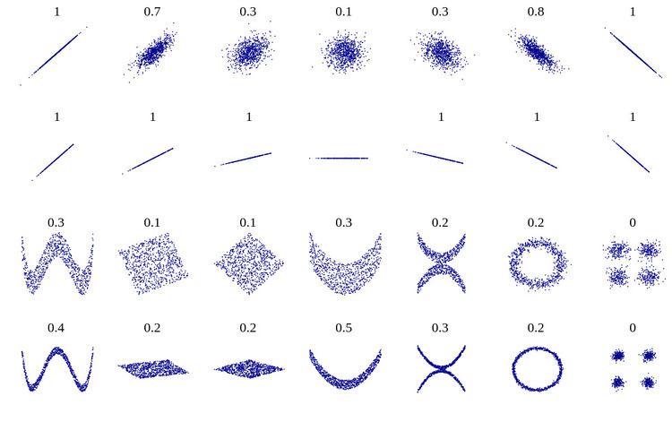
The classical measure of dependence, the Pearson correlation coefficient, is mainly sensitive to a linear relationship between two variables. Distance correlation was introduced in 2005 by Gabor J Szekely in several lectures to address this deficiency of Pearson’s correlation, namely that it can easily be zero for dependent variables. Correlation = 0 (uncorrelatedness) does not imply independence while distance correlation = 0 does imply independence. The first results on distance correlation were published in 2007 and 2009. It was proved that distance covariance is the same as the Brownian covariance. These measures are examples of energy distances.

Distance covariance

Let us start with the definition of the sample distance covariance. Let (X_k, Y_k), k= 1, 2, ..., n be a statistical sample from a pair of real valued or vector valued random variables (X, Y). First, compute the n by n distance matrices (a_{j, k}) and (b_{j, k}) containing all pairwise distances

where || ⋅ || denotes Euclidean norm. Then take all doubly centered distances

where a ¯ j . is the j-th row mean, a ¯ . k is the k-th column mean, and a ¯ . . is the grand mean of the distance matrix of the X sample. The notation is similar for the b values. (In the matrices of centered distances (A_{j, k}) and (B_j,k) all rows and all columns sum to zero.) The squared sample distance covariance (a scalar) is simply the arithmetic average of the products A_{j, k} B_{j, k}:

The statistic T_n = n dCov²_n(X, Y) determines a consistent multivariate test of independence of random vectors in arbitrary dimensions. For an implementation see dcov.test function in the energy package for R.

The population value of distance covariance can be defined along the same lines. Let X be a random variable that takes values in a p-dimensional Euclidean space with probability distribution μ and let Y be a random variable that takes values in a q-dimensional Euclidean space with probability distribution ν, and suppose that X and Y have finite expectations. Write

Finally, define the population value of squared distance covariance of X and Y as

One can show that this is equivalent to the following definition:

where E denotes expected value, and ( X , Y ) , ( X ′ , Y ′ ) , and ( X ″ , Y ″ ) are independent and identically distributed. Distance covariance can be expressed in terms of the classical Pearson’s covariance, cov, as follows:

This identity shows that the distance covariance is not the same as the covariance of distances, cov(||X-X' ||, ||Y-Y' ||). This can be zero even if X and Y are not independent.

Alternatively, the squared distance covariance can be defined as the weighted L² norm of the distance between the joint characteristic function of the random variables and the product of their marginal characteristic functions:

dCov 2 ⁡ ( X , Y ) = 1 c p c q ∫ R p + q | ϕ X , Y ( s , t ) − ϕ X ( s ) ϕ Y ( t ) | 2 | s | p 1 + p | t | q 1 + q d t d s

where ϕ_{X, Y}(s, t), ϕ_X(s), and ϕ_Y(t) are the characteristic functions of (X, Y), X, and Y, respectively, p, q denote the Euclidean dimension of X and Y, and thus of s and t, and c_p, c_q are constants. The weight function ( c p c q | s | p 1 + p | t | q 1 + q ) − 1 is chosen to produce a scale equivariant and rotation invariant measure that doesn't go to zero for dependent variables. One interpretation of the characteristic function definition is that the variables e^isX and e^itY are cyclic representations of X and Y with different periods given by s and t, and the expression ϕ_{X, Y}(s, t) - ϕ_X(s) ϕ_Y(t) in the numerator of the characteristic function definition of distance covariance is simply the classical covariance of e^isX and e^itY. The characteristic function definition clearly shows that dCov²(X, Y) = 0 if and only if X and Y are independent.

Distance variance and standard deviation

The distance variance is a special case of distance covariance when the two variables are identical. The population value of distance variance is the square root of

where E denotes the expected value, X ′ is an independent and identically distributed copy of X and X ″ is independent of X and X ′ and has the same distribution as X and X ′ .

The sample distance variance is the square root of

which is a relative of Corrado Gini’s mean difference introduced in 1912 (but Gini did not work with centered distances).

The distance standard deviation is the square root of the distance variance.

Distance correlation

The distance correlation of two random variables is obtained by dividing their distance covariance by the product of their distance standard deviations. The distance correlation is

and the sample distance correlation is defined by substituting the sample distance covariance and distance variances for the population coefficients above.

For easy computation of sample distance correlation see the dcor function in the energy package for R.

Distance correlation

(i) 0 ≤ dCor n ⁡ ( X , Y ) ≤ 1 and 0 ≤ dCor ⁡ ( X , Y ) ≤ 1 ; this is in contrast to Person's correlation, which can be negative.

(ii) dCor ⁡ ( X , Y ) = 0 if and only if X and Y are independent.

(iii) dCor n ⁡ ( X , Y ) = 1 implies that dimensions of the linear subspaces spanned by X and Y samples respectively are almost surely equal and if we assume that these subspaces are equal, then in this subspace Y = A + b C X for some vector A , scalar b , and orthonormal matrix C .

Distance covariance

(i) dCov ⁡ ( X , Y ) ≥ 0 and dCov n ⁡ ( X , Y ) ≥ 0 ;

(ii) dCov 2 ⁡ ( a 1 + b 1 C 1 X , a 2 + b 2 C 2 Y ) = | b 1 b 2 | dCov 2 ⁡ ( X , Y ) for all constant vectors a 1 , a 2 , scalars b 1 , b 2 , and orthonormal matrices C 1 , C 2 .

(iii) If the random vectors ( X 1 , Y 1 ) and ( X 2 , Y 2 ) are independent then

Equality holds if and only if X 1 and Y 1 are both constants, or X 2 and Y 2 are both constants, or X 1 , X 2 , Y 1 , Y 2 are mutually independent.

(iv) dCov ⁡ ( X , Y ) = 0 if and only if X and Y are independent.

This last property is the most important effect of working with centered distances.

The statistic dCov n 2 ⁡ ( X , Y ) is a biased estimator of dCov 2 ⁡ ( X , Y ) . Under independence of X and Y

An unbiased estimator of dCov 2 ⁡ ( X , Y ) is given by Székely and Rizzo.

Distance variance

(i) dVar ⁡ ( X ) = 0 if and only if X = E ⁡ [ X ] almost surely.

(ii) dVar n ⁡ ( X ) = 0 if and only if every sample observation is identical.

(iii) dVar ⁡ ( A + b C X ) = | b | dVar ⁡ ( X ) for all constant vectors A , scalars b , and orthonormal matrices C .

(iv) If X and Y are independent then dVar ⁡ ( X + Y ) ≤ dVar ⁡ ( X ) + dVar ⁡ ( Y ) .

Equality holds in (iv) if and only if one of the random variables X or Y is a constant.

Generalization

Distance covariance can be generalized to include powers of Euclidean distance. Define

Then for every 0 < α < 2 , X and Y are independent if and only if dCov 2 ⁡ ( X , Y ; α ) = 0 . It is important to note that this characterization does not hold for exponent α = 2 ; in this case for bivariate ( X , Y ) , dCor ⁡ ( X , Y ; α = 2 ) is a deterministic function of the Pearson correlation. If a k , ℓ and b k , ℓ are α powers of the corresponding distances, 0 < α ≤ 2 , then α sample distance covariance can be defined as the nonnegative number for which

One can extend dCov to metric-space-valued random variables X and Y : If X has law μ in a metric space with metric d , then define a μ ( x ) := E ⁡ [ d ( X , x ) ] , D ( μ ) := E ⁡ [ a μ ( X ) ] , and (provided a μ is finite, i.e., X has finite first moment), d μ ( x , x ′ ) := d ( x , x ′ ) − a μ ( x ) − a μ ( x ′ ) + D ( μ ) . Then if Y has law ν (in a possibly different metric space with finite first moment), define

This is non-negative for all such X , Y iff both metric spaces have negative type. Here, a metric space ( M , d ) has negative type if ( M , d 1 / 2 ) is isometric to a subset of a Hilbert space. If both metric spaces have strong negative type, then dCov 2 ⁡ ( X , Y ) = 0 iff X , Y are independent.

Alternative definition of distance covariance

The original distance covariance has been defined as the square root of dCov 2 ⁡ ( X , Y ) , rather than the squared coefficient itself. dCov ⁡ ( X , Y ) has the property that it is the energy distance between the joint distribution of X , Y and the product of its marginals. Under this definition, however, the distance variance, rather than the distance standard deviation, is measured in the same units as the X distances.

Alternately, one could define distance covariance to be the square of the energy distance: dCov 2 ⁡ ( X , Y ) . In this case, the distance standard deviation of X is measured in the same units as X distance, and there exists an unbiased estimator for the population distance covariance.

Under these alternate definitions, the distance correlation is also defined as the square dCor 2 ⁡ ( X , Y ) , rather than the square root.

Alternative formulation: Brownian covariance

Brownian covariance is motivated by generalization of the notion of covariance to stochastic processes. The square of the covariance of random variables X and Y can be written in the following form:

where E denotes the expected value and the prime denotes independent and identically distributed copies. We need the following generalization of this formula. If U(s), V(t) are arbitrary random processes defined for all real s and t then define the U-centered version of X by

whenever the subtracted conditional expected value exists and denote by Y_V the V-centered version of Y. The (U,V) covariance of (X,Y) is defined as the nonnegative number whose square is

whenever the right-hand side is nonnegative and finite. The most important example is when U and V are two-sided independent Brownian motions /Wiener processes with expectation zero and covariance |s| + |t| - |s-t| = 2 min(s,t) (for nonnegative s, t only). (This is twice the covariance of the standard Wiener process; here the factor 2 simplifies the computations.) In this case the (U,V) covariance is called Brownian covariance and is denoted by

There is a surprising coincidence: The Brownian covariance is the same as the distance covariance:

and thus Brownian correlation is the same as distance correlation.

On the other hand, if we replace the Brownian motion with the deterministic identity function id then Cov_id(X,Y) is simply the absolute value of the classical Pearson covariance,