
 | ||
Binary or binomial classification is the task of classifying the elements of a given set into two groups on the basis of a classification rule. Instancing a decision whether an item has or not some qualitative property, some specified characteristic, some typical binary classification tasks are:
Contents
- Statistical binary classification
- Evaluation of binary classifiers
- Converting continuous values to binary
- References
Binary classification is dichotomization applied to practical purposes, and therefore an important point is that in many practical binary classification problems, the two groups are not symmetric – rather than overall accuracy, the relative proportion of different types of errors is of interest. For example, in medical testing, a false positive (detecting a disease when it is not present) is considered differently from a false negative (not detecting a disease when it is present).
Porting human discriminative abilities to scientific soundness and technical practice is far from trivial.
Statistical binary classification
Statistical classification is a problem studied in machine learning. It is a type of supervised learning, a method of machine learning where the categories are predefined, and is used to categorize new probabilistic observations into said categories. When there are only two categories the problem is known as statistical binary classification.
Some of the methods commonly used for binary classification are:
Each classifier is best in only a select domain based upon the number of observations, the dimensionality of the feature vector, the noise in the data and many other factors. For example random forests perform better than SVM classifiers for 3D point clouds.
Evaluation of binary classifiers
There are many metrics that can be used to measure the performance of a classifier or predictor; different fields have different preferences for specific metrics due to different goals. For example, in medicine sensitivity and specificity are often used, while in information retrieval precision and recall are preferred. An important distinction is between metrics that are independent on the prevalence (how often each category occurs in the population), and metrics that depend on the prevalence – both types are useful, but they have very different properties.
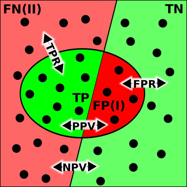
Given a classification of a specific data set, there are four basic data: the number of true positives (TP), true negatives (TN), false positives (FP), and false negatives (FN). These can be arranged into a 2×2 contingency table, with columns corresponding to actual value – condition positive (CP) or condition negative (CN) – and rows corresponding to classification value – test outcome positive or test outcome negative. There are eight basic ratios that one can compute from this table, which come in four complementary pairs (each pair summing to 1). These are obtained by dividing each of the four numbers by the sum of its row or column, yielding eight numbers, which can be referred to generically in the form "true positive row ratio" or "false negative column ratio", though there are conventional terms. There are thus two pairs of column ratios and two pairs of row ratios, and one can summarize these with four numbers by choosing one ratio from each pair – the other four numbers are the complements.
The column ratios are True Positive Rate (TPR, aka Sensitivity or recall), with complement the False Negative Rate (FNR); and True Negative Rate (TNR, aka Specificity, SPC), with complement False Positive Rate (FPR). These are the proportion of the population with the condition (resp., without the condition) for which the test is correct (or, complementarily, for which the test is incorrect); these are independent of prevalence.
The row ratios are Positive Predictive Value (PPV, aka precision), with complement the False Discovery Rate (FDR); and Negative Predictive Value (NPV), with complement the False Omission Rate (FOR). These are the proportion of the population with a given test result for which the test is correct (or, complementarily, for which the test is incorrect); these depend on prevalence.
In diagnostic testing, the main ratios used are the true column ratios – True Positive Rate and True Negative Rate – where they are known as sensitivity and specificity. In informational retrieval, the main ratios are the true positive ratios (row and column) – Positive Predictive Value and True Positive Rate – where they are known as precision and recall.
One can take ratios of a complementary pair of ratios, yielding four likelihood ratios (two column ratio of ratios, two row ratio of ratios). This is primarily done for the column (condition) ratios, yielding likelihood ratios in diagnostic testing. Taking the ratio of one of these groups of ratios yields a final ratio, the diagnostic odds ratio (DOR). This can also be defined directly as (TP×TN)/(FP×FN) = (TP/FN)/(FP/TN); this has a useful interpretation – as an odds ratio – and is prevalence-independent.
There are a number of other metrics, most simply the accuracy or Fraction Correct (FC), which measures the fraction of all instances that are correctly categorized; the complement is the Fraction Incorrect (FiC). The F-score combines precision and recall into one number via a choice of weighing, most simply equal weighing, as the balanced F-score (F1 score). Some metrics come from regression coefficients: the markedness and the informedness, and their geometric mean, the Matthews correlation coefficient. Other metrics include Youden's J statistic, the uncertainty coefficient, the Phi coefficient, and Cohen's kappa.
Converting continuous values to binary
Tests whose results are of continuous values, such as most blood values, can artificially be made binary by defining a cutoff value, with test results being designated as positive or negative depending on whether the resultant value is higher or lower than the cutoff.
However, such conversion causes a loss of information, as the resultant binary classification does not tell how much above or below the cutoff a value is. As a result, when converting a continuous value that is close to the cutoff to a binary one, the resultant positive or negative predictive value is generally higher than the predictive value given directly from the continuous value. In such cases, the designation of the test of being either positive or negative gives the appearance of an inappropriately high certainty, while the value is in fact in an interval of uncertainty. For example, with the urine concentration of hCG as a continuous value, a urine pregnancy test that measured 52 mIU/ml of hCG may show as "positive" with 50 mIU/ml as cutoff, but is in fact in an interval of uncertainty, which may be apparent only by knowing the original continuous value. On the other hand, a test result very far from the cutoff generally has a resultant positive or negative predictive value that is lower than the predictive value given from the continuous value. For example, a urine hCG value of 200,000 mIU/ml confers a very high probability of pregnancy, but conversion to binary values results in that it shows just as "positive" as the one of 52 mIU/ml.