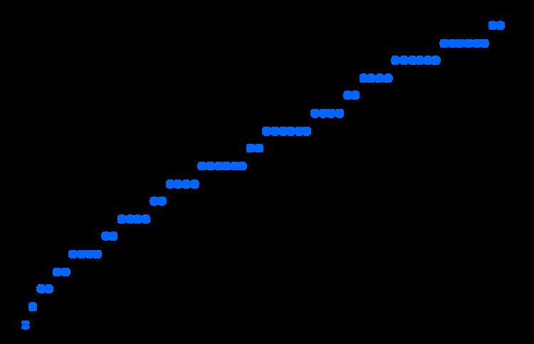
Prime counting function - Alchetron, the free social encyclopedia

In mathematics, the prime-counting function is the function counting the number of prime numbers less than or equal to some real number x. It is denoted by π(x) (unrelated to the number π).

History

Of great interest in number theory is the growth rate of the prime-counting function. It was conjectured in the end of the 18th century by Gauss and by Legendre to be approximately

x ln ⁡ ( x )

in the sense that

lim x → ∞ π ( x ) x / ln ⁡ ( x ) = 1.

This statement is the prime number theorem. An equivalent statement is

lim x → ∞ π ( x ) / li ⁡ ( x ) = 1

where li is the logarithmic integral function. The prime number theorem was first proved in 1896 by Jacques Hadamard and by Charles de la Vallée Poussin independently, using properties of the Riemann zeta function introduced by Riemann in 1859.

More precise estimates of π ( x ) are now known; for example

π ( x ) = li ⁡ ( x ) + O ( x e − ln ⁡ x / 15 )

where the O is big O notation. For most values of x we are interested in (i.e., when x is not unreasonably large) li ⁡ ( x ) is greater than π ( x ) , but infinitely often the opposite is true. For a discussion of this, see Skewes' number.

Proofs of the prime number theorem not using the zeta function or complex analysis were found around 1948 by Atle Selberg and by Paul Erdős (for the most part independently).

Table of π(x), x / ln x, and li(x)

The table shows how the three functions π(x), x / ln x and li(x) compare at powers of 10. See also, and

In the On-Line Encyclopedia of Integer Sequences, the π(x) column is sequence A006880, π(x) − x/ln x is sequence A057835, and li(x) − π(x) is sequence A057752.

The value for π(10²⁴) was originally computed by J. Buethe, J. Franke, A. Jost, and T. Kleinjung assuming the Riemann hypothesis. It was later verified unconditionally in a computation by D. J. Platt. The value for π(10²⁵) is due to J. Buethe, J. Franke, A. Jost, and T. Kleinjung. The value for π(10²⁶) was computed by D. B. Staple. All other entries in this table were also verified as part of that work.

Algorithms for evaluating π(x)

A simple way to find π ( x ) , if x is not too large, is to use the sieve of Eratosthenes to produce the primes less than or equal to x and then to count them.

A more elaborate way of finding π ( x ) is due to Legendre: given x , if p 1 , p 2 , … , p n are distinct prime numbers, then the number of integers less than or equal to x which are divisible by no p i is

⌊ x ⌋ − ∑ i ⌊ x p i ⌋ + ∑ i < j ⌊ x p i p j ⌋ − ∑ i < j < k ⌊ x p i p j p k ⌋ + ⋯

(where ⌊ ⋯ ⌋ denotes the floor function). This number is therefore equal to

π ( x ) − π ( x ) + 1

when the numbers p 1 , p 2 , … , p n are the prime numbers less than or equal to the square root of x .

The Meissel–Lehmer algorithm

In a series of articles published between 1870 and 1885, Ernst Meissel described (and used) a practical combinatorial way of evaluating π ( x ) . Let p 1 , p 2 , … , p n be the first n primes and denote by Φ ( m , n ) the number of natural numbers not greater than m which are divisible by no p i . Then

Φ ( m , n ) = Φ ( m , n − 1 ) − Φ ( m p n , n − 1 ) .

Given a natural number m , if n = π ( m 3 ) and if μ = π ( m ) − n , then

π ( m ) = Φ ( m , n ) + n ( μ + 1 ) + μ 2 − μ 2 − 1 − ∑ k = 1 μ π ( m p n + k ) .

Using this approach, Meissel computed π ( x ) , for x equal to 5×10⁵, 10⁶, 10⁷, and 10⁸.

In 1959, Derrick Henry Lehmer extended and simplified Meissel's method. Define, for real m and for natural numbers n and k , P k ( m , n ) as the number of numbers not greater than m with exactly k prime factors, all greater than p n . Furthermore, set P 0 ( m , n ) = 1 . Then

Φ ( m , n ) = ∑ k = 0 + ∞ P k ( m , n )

where the sum actually has only finitely many nonzero terms. Let y denote an integer such that m 3 ≤ y ≤ m , and set n = π ( y ) . Then P 1 ( m , n ) = π ( m ) − n and P k ( m , n ) = 0 when k ≥ 3. Therefore,

π ( m ) = Φ ( m , n ) + n − 1 − P 2 ( m , n )

The computation of P 2 ( m , n ) can be obtained this way:

P 2 ( m , n ) = ∑ y < p ≤ m ( π ( m p ) − π ( p ) + 1 ) ,

where the sum is over prime numbers.

On the other hand, the computation of Φ ( m , n ) can be done using the following rules:

Φ ( m , 0 ) = ⌊ m ⌋
Φ ( m , b ) = Φ ( m , b − 1 ) − Φ ( m p b , b − 1 )

Using his method and an IBM 701, Lehmer was able to compute π ( 10 10 ) .

Further improvements to this method were made by Lagarias, Miller, Odlyzko, Deléglise and Rivat.

Other prime-counting functions

Other prime-counting functions are also used because they are more convenient to work with. One is Riemann's prime-counting function, usually denoted as Π 0 ( x ) or J 0 ( x ) . This has jumps of 1/n for prime powers pⁿ, with it taking a value halfway between the two sides at discontinuities. That added detail is because then it may be defined by an inverse Mellin transform. Formally, we may define Π 0 ( x ) by

Π 0 ( x ) = 1 2 ( ∑ p n < x 1 n + ∑ p n ≤ x 1 n )

where p is a prime.

We may also write

Π 0 ( x ) = ∑ 2 x Λ ( n ) ln ⁡ n − 1 2 Λ ( x ) ln ⁡ x = ∑ n = 1 ∞ 1 n π 0 ( x 1 / n )

where Λ(n) is the von Mangoldt function and

π 0 ( x ) = lim ε → 0 π ( x − ε ) + π ( x + ε ) 2 .

The Möbius inversion formula then gives

π 0 ( x ) = ∑ n = 1 ∞ μ ( n ) n Π 0 ( x 1 / n )

Knowing the relationship between log of the Riemann zeta function and the von Mangoldt function Λ , and using the Perron formula we have

ln ⁡ ζ ( s ) = s ∫ 0 ∞ Π 0 ( x ) x − s − 1 d x

The Chebyshev function weights primes or prime powers pⁿ by ln(p):

θ ( x ) = ∑ p ≤ x ln ⁡ p ψ ( x ) = ∑ p n ≤ x ln ⁡ p = ∑ n = 1 ∞ θ ( x 1 / n ) = ∑ n ≤ x Λ ( n ) .

Formulas for prime-counting functions

Formulas for prime-counting functions come in two kinds: arithmetic formulas and analytic formulas. Analytic formulas for prime-counting were the first used to prove the prime number theorem. They stem from the work of Riemann and von Mangoldt, and are generally known as explicit formulas.

We have the following expression for ψ:

ψ 0 ( x ) = x − ∑ ρ x ρ ρ − ln ⁡ 2 π − 1 2 ln ⁡ ( 1 − x − 2 )

where

ψ 0 ( x ) = lim ε → 0 ψ ( x − ε ) + ψ ( x + ε ) 2 .

Here ρ are the zeros of the Riemann zeta function in the critical strip, where the real part of ρ is between zero and one. The formula is valid for values of x greater than one, which is the region of interest. The sum over the roots is conditionally convergent, and should be taken in order of increasing absolute value of the imaginary part. Note that the same sum over the trivial roots gives the last subtrahend in the formula.

For Π 0 ( x ) we have a more complicated formula

Π 0 ( x ) = li ⁡ ( x ) − ∑ ρ li ⁡ ( x ρ ) − ln ⁡ 2 + ∫ x ∞ d t t ( t 2 − 1 ) ln ⁡ t .

Again, the formula is valid for x > 1, while ρ are the nontrivial zeros of the zeta function ordered according to their absolute value, and, again, the latter integral, taken with minus sign, is just the same sum, but over the trivial zeros. The first term li(x) is the usual logarithmic integral function; the expression li(x^ρ) in the second term should be considered as Ei(ρ ln x), where Ei is the analytic continuation of the exponential integral function from positive reals to the complex plane with branch cut along the negative reals.

Thus, Möbius inversion formula gives us

π 0 ( x ) = R ⁡ ( x ) − ∑ ρ R ⁡ ( x ρ ) − 1 ln ⁡ x + 1 π arctan ⁡ π ln ⁡ x

valid for x > 1, where

R ⁡ ( x ) = ∑ n = 1 ∞ μ ( n ) n li ⁡ ( x 1 / n ) = 1 + ∑ k = 1 ∞ ( ln ⁡ x ) k k ! k ζ ( k + 1 )

is so-called Riemann's R-function. The latter series for it is known as Gram series and converges for all positive x.

The sum over non-trivial zeta zeros in the formula for π 0 ( x ) describes the fluctuations of π 0 ( x ) , while the remaining terms give the "smooth" part of prime-counting function, so one can use

R ⁡ ( x ) − 1 ln ⁡ x + 1 π arctan ⁡ π ln ⁡ x

as the best estimator of π ( x ) for x > 1.

The amplitude of the "noisy" part is heuristically about x / ln ⁡ x , so the fluctuations of the distribution of primes may be clearly represented with the Δ-function:

Δ ( x ) = ( π 0 ( x ) − R ⁡ ( x ) + 1 ln ⁡ x − 1 π arctan ⁡ π ln ⁡ x ) ln ⁡ x x .

An extensive table of the values of Δ(x) is available.

Inequalities

Here are some useful inequalities for π(x).

x ln ⁡ x < π ( x ) < 1.25506 x ln ⁡ x

for x ≥ 17. The left inequality holds for x ≥ 17 and the right inequality holds for x > 1.

An explanation of the constant 1.25506 is given at (sequence A209883 in the OEIS).

Pierre Dusart proved in 2010:

x ln ⁡ x − 1 < π ( x ) for x ≥ 5393 , and π ( x ) < x ln ⁡ x − 1.1 for x ≥ 60184 .

Here are some inequalities for the nth prime, p_n.

n ( ln ⁡ ( n ln ⁡ n ) − 1 ) < p n < n ln ⁡ ( n ln ⁡ n ) for n ≥ 6.

The left inequality holds for n ≥ 1 and the right inequality holds for n ≥ 6.

An approximation for the nth prime number is

p n = n ( ln ⁡ ( n ln ⁡ n ) − 1 ) + n ( ln ⁡ ln ⁡ n − 2 ) ln ⁡ n + O ( n ( ln ⁡ ln ⁡ n ) 2 ( ln ⁡ n ) 2 ) .

In his well-known notebooks, Ramanujan proves that the inequality

π ( x ) 2 < e x log ⁡ x π ( x e )

holds for all sufficiently large values of x .

The Riemann hypothesis

The Riemann hypothesis is equivalent to a much tighter bound on the error in the estimate for π ( x ) , and hence to a more regular distribution of prime numbers,

π ( x ) = li ⁡ ( x ) + O ( x log ⁡ x ) .

Specifically,

| π ( x ) − li ⁡ ( x ) | < 1 8 π x log ⁡ x , for all x ≥ 2657.

References

Prime-counting function Wikipedia

(Text) CC BY-SA

Contents