Chebyshev function - Alchetron, The Free Social Encyclopedia

In mathematics, the Chebyshev function is either of two related functions. The first Chebyshev function ϑ(x) or θ(x) is given by

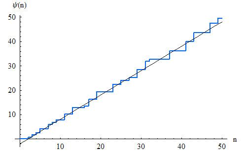
where Λ is the von Mangoldt function. The Chebyshev functions, especially the second one ψ(x), are often used in proofs related to prime numbers, because it is typically simpler to work with them than with the prime-counting function, π(x) (See the exact formula, below.) Both Chebyshev functions are asymptotic to x, a statement equivalent to the prime number theorem.

Both functions are named in honour of Pafnuty Chebyshev.

Relationships

The second Chebyshev function can be seen to be related to the first by writing it as

ψ ( x ) = ∑ p ≤ x k log ⁡ p

where k is the unique integer such that p^k ≤ x and x < p^{k + 1}. The values k of are given in A206722. A more direct relationship is given by

ψ ( x ) = ∑ n = 1 ∞ ϑ ( x 1 n ) .

Note that this last sum has only a finite number of non-vanishing terms, as

ϑ ( x 1 n ) = 0 for n > log 2 ⁡ x = log ⁡ x log ⁡ 2 .

The second Chebyshev function is the logarithm of the least common multiple of the integers from 1 to n.

lcm ⁡ ( 1 , 2 , … , n ) = e ψ ( n ) .

Values of lcm(1,2,...,n) for the integer variable n is given at A003418.

Asymptotics and bounds

The following bounds are known for the Chebyshev functions:^[1]^[2] (in these formulas p_k is the kth prime number p₁ = 2, p₂ = 3, etc.)

ϑ ( p k ) ≥ k ( ln ⁡ k + ln ⁡ ln ⁡ k − 1 + ln ⁡ ln ⁡ k − 2.050735 ln ⁡ k ) for k ≥ 10 11 , ϑ ( p k ) ≤ k ( ln ⁡ k + ln ⁡ ln ⁡ k − 1 + ln ⁡ ln ⁡ k − 2 ln ⁡ k ) for k ≥ 198 , | ϑ ( x ) − x | ≤ 0.006788 x ln ⁡ x for x ≥ 10 544 111 , | ψ ( x ) − x | ≤ 0.006409 x ln ⁡ x for x ≥ e 22 , 0.9999 x < ψ ( x ) − ϑ ( x ) < 1.00007 x + 1.78 x 3 for x ≥ 121.

Furthermore, under the Riemann hypothesis,

| ϑ ( x ) − x | = O ( x 1 2 + ε ) | ψ ( x ) − x | = O ( x 1 2 + ε )

for any ε > 0.

Upper bounds exist for both ϑ(x) and ψ(x) such that, ^[3]

ϑ ( x ) < 1.000028 x ψ ( x ) < 1.03883 x

for any x > 0.

An explanation of the constant 1.03883 is given at A206431.

The exact formula

In 1895, Hans Carl Friedrich von Mangoldt proved^[4] an explicit expression for ψ(x) as a sum over the nontrivial zeros of the Riemann zeta function:

ψ 0 ( x ) = x − ∑ ρ x ρ ρ − ζ ′ ( 0 ) ζ ( 0 ) − 1 2 log ⁡ ( 1 − x − 2 ) .

(The numerical value of ζ′(0)/ζ(0) is log(2π).) Here ρ runs over the nontrivial zeros of the zeta function, and ψ₀ is the same as ψ, except that at its jump discontinuities (the prime powers) it takes the value halfway between the values to the left and the right:

ψ 0 ( x ) = 1 2 ( ∑ n ≤ x Λ ( n ) + ∑ n < x Λ ( n ) ) = { ψ ( x ) − 1 2 Λ ( x ) x = 2 , 3 , 4 , 5 , 7 , 8 , 9 , 11 , 13 , 16 , … ψ ( x ) otherwise.

From the Taylor series for the logarithm, the last term in the explicit formula can be understood as a summation of x^ω/ω over the trivial zeros of the zeta function, ω = −2, −4, −6, ..., i.e.

∑ k = 1 ∞ x − 2 k − 2 k = 1 2 log ⁡ ( 1 − x − 2 ) .

Similarly, the first term, x = x¹/1, corresponds to the simple pole of the zeta function at 1. Its being a pole rather than zero accounts for the opposite sign of the term.

Properties

A theorem due to Erhard Schmidt states that, for some explicit positive constant K, there are infinitely many natural numbers x such that

ψ ( x ) − x < − K x

and infinitely many natural numbers x such that

ψ ( x ) − x > K x . ^[5]^[6]

In little-o notation, one may write the above as

ψ ( x ) − x ≠ o ( x ) .

Hardy and Littlewood^[7] prove the stronger result, that

ψ ( x ) − x ≠ o ( x log ⁡ log ⁡ log ⁡ x ) .

Relation to primorials

The first Chebyshev function is the logarithm of the primorial of x, denoted x#:

ϑ ( x ) = ∑ p ≤ x log ⁡ p = log ⁡ ∏ p ≤ x p = log ⁡ ( x # ) .

This proves that the primorial x# is asymptotically equal to e^{(1 + o(1))x}, where "o" is the little-o notation (see big O notation) and together with the prime number theorem establishes the asymptotic behavior of p_n#.

Relation to the prime-counting function

The Chebyshev function can be related to the prime-counting function as follows. Define

Π ( x ) = ∑ n ≤ x Λ ( n ) log ⁡ n .

Then

Π ( x ) = ∑ n ≤ x Λ ( n ) ∫ n x d t t log 2 ⁡ t + 1 log ⁡ x ∑ n ≤ x Λ ( n ) = ∫ 2 x ψ ( t ) d t t log 2 ⁡ t + ψ ( x ) log ⁡ x .

The transition from Π to the prime-counting function, π, is made through the equation

Π ( x ) = π ( x ) + 1 2 π ( x ) + 1 3 π ( x 3 ) + ⋯

Certainly π(x) ≤ x, so for the sake of approximation, this last relation can be recast in the form

π ( x ) = Π ( x ) + O ( x ) .

The Riemann hypothesis

The Riemann hypothesis states that all nontrivial zeros of the zeta function have real part 1/2. In this case, | x^ρ | = √x, and it can be shown that

∑ ρ x ρ ρ = O ( x log 2 ⁡ x ) .

By the above, this implies

π ( x ) = li ⁡ ( x ) + O ( x log ⁡ x ) .

Good evidence that the hypothesis could be true comes from the fact proposed by Alain Connes and others, that if we differentiate the von Mangoldt formula with respect to x we get x = e^u. Manipulating, we have the "Trace formula" for the exponential of the Hamiltonian operator satisfying

ζ ( 1 2 + i H ^ ) | n ≥ ζ ( 1 2 + i E n ) = 0 ,

and

∑ n e i u E n = Z ( u ) = e u 2 − e − u 2 d ψ 0 d u − e u 2 e 3 u − e u = Tr ⁡ ( e i u H ^ ) ,

where the "trigonometric sum" can be considered to be the trace of the operator (statistical mechanics) e^iuĤ, which is only true if ρ = 1/2 + iE(n).

Using the semiclassical approach the potential of H = T + V satisfies:

Z ( u ) u 1 2 π ∼ ∫ − ∞ ∞ e i ( u V ( x ) + π 4 ) d x

with Z(u) → 0 as u → ∞.

solution to this nonlinear integral equation can be obtained (among others) by

V − 1 ( x ) ≈ 4 π ⋅ d 1 2 d x 1 2 N ( x )

in order to obtain the inverse of the potential:

π N ( E ) = Arg ⁡ ξ ( 1 2 + i E ) .

Smoothing function

The smoothing function is defined as

ψ 1 ( x ) = ∫ 0 x ψ ( t ) d t .

It can be shown that

ψ 1 ( x ) ∼ x 2 2 .

Variational formulation

The Chebyshev function evaluated at x = e^t minimizes the functional

J [ f ] = ∫ 0 ∞ f ( s ) ζ ′ ( s + c ) ζ ( s + c ) ( s + c ) d s − ∫ 0 ∞ ∫ 0 ∞ e − s t f ( s ) f ( t ) d s d t ,

so

f ( t ) = ψ ( e t ) e − c t for c > 0.

References

Chebyshev function Wikipedia

(Text) CC BY-SA

Contents