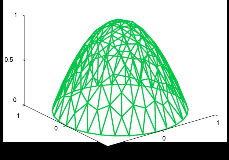
Discretization - Alchetron, The Free Social Encyclopedia

In mathematics, discretization concerns the process of transferring continuous functions, models, and equations into discrete counterparts. This process is usually carried out as a first step toward making them suitable for numerical evaluation and implementation on digital computers. Dichotomization is the special case of discretization in which the number of discrete classes is 2, which can approximate a continuous variable as a binary variable (creating a dichotomy for modeling purposes, as in binary classification).

Discretization is also related to discrete mathematics, and is an important component of granular computing. In this context, discretization may also refer to modification of variable or category granularity, as when multiple discrete variables are aggregated or multiple discrete categories fused.

Whenever continuous data is discretized, there is always some amount of discretization error. The goal is to reduce the amount to a level considered negligible for the modeling purposes at hand.

Discretization is not always distinguished from quantization in any clearly defined way. The two terms share a semantic field. The same is true of discretization error and quantization error.

Mathematical methods relating to discretization include the Euler–Maruyama method and the zero-order hold.

Discretization of linear state space models

Discretization is also concerned with the transformation of continuous differential equations into discrete difference equations, suitable for numerical computing.

The following continuous-time state space model

x ˙ ( t ) = A x ( t ) + B u ( t ) + w ( t ) y ( t ) = C x ( t ) + D u ( t ) + v ( t )

where v and w are continuous zero-mean white noise sources with covariances

w ( t ) ∼ N ( 0 , Q ) v ( t ) ∼ N ( 0 , R )

can be discretized, assuming zero-order hold for the input u and continuous integration for the noise v, to

x [ k + 1 ] = A d x [ k ] + B d u [ k ] + w [ k ] y [ k ] = C d x [ k ] + D d u [ k ] + v [ k ]

with covariances

w [ k ] ∼ N ( 0 , Q d ) v [ k ] ∼ N ( 0 , R d )

where

A d = e A T = L − 1 { ( s I − A ) − 1 } t = T B d = ( ∫ τ = 0 T e A τ d τ ) B = A − 1 ( A d − I ) B , if A is nonsingular C d = C D d = D Q d = ∫ τ = 0 T e A τ Q e A T τ d τ R d = 1 T R

and T is the sample time, although A T is the transposed matrix of A .

A clever trick to compute A_d and B_d in one step is by utilizing the following property:

e [ A B 0 0 ] T = [ M 11 M 12 0 I ]

and then having

A d = M 11 B d = M 12

Discretization of process noise

Numerical evaluation of Q d is a bit trickier due to the matrix exponential integral. It can, however, be computed by first constructing a matrix, and computing the exponential of it (Van Loan, 1978):

F = [ − A Q 0 A T ] T G = e F = [ … A d − 1 Q d 0 A d T ] .

The discretized process noise is then evaluated by multiplying the transpose of the lower-right partition of G with the upper-right partition of G:

Q d = ( A d T ) T ( A d − 1 Q d ) .

Derivation

Starting with the continuous model

x ˙ ( t ) = A x ( t ) + B u ( t )

we know that the matrix exponential is

d d t e A t = A e A t = e A t A

and by premultiplying the model we get

e − A t x ˙ ( t ) = e − A t A x ( t ) + e − A t B u ( t )

which we recognize as

d d t ( e − A t x ( t ) ) = e − A t B u ( t )

and by integrating..

e − A t x ( t ) − e 0 x ( 0 ) = ∫ 0 t e − A τ B u ( τ ) d τ x ( t ) = e A t x ( 0 ) + ∫ 0 t e A ( t − τ ) B u ( τ ) d τ

which is an analytical solution to the continuous model.

Now we want to discretise the above expression. We assume that u is constant during each timestep.

x [ k ] = d e f x ( k T ) x [ k ] = e A k T x ( 0 ) + ∫ 0 k T e A ( k T − τ ) B u ( τ ) d τ x [ k + 1 ] = e A ( k + 1 ) T x ( 0 ) + ∫ 0 ( k + 1 ) T e A ( ( k + 1 ) T − τ ) B u ( τ ) d τ x [ k + 1 ] = e A T [ e A k T x ( 0 ) + ∫ 0 k T e A ( k T − τ ) B u ( τ ) d τ ] + ∫ k T ( k + 1 ) T e A ( k T + T − τ ) B u ( τ ) d τ

We recognize the bracketed expression as x [ k ] , and the second term can be simplified by substituting v = k T + T − τ . We also assume that u is constant during the integral, which in turn yields

x [ k + 1 ] = e A T x [ k ] + ( ∫ 0 T e A v d v ) B u [ k ] = e A T x [ k ] + A − 1 ( e A T − I ) B u [ k ]

which is an exact solution to the discretization problem.

Approximations

Exact discretization may sometimes be intractable due to the heavy matrix exponential and integral operations involved. It is much easier to calculate an approximate discrete model, based on that for small timesteps e A T ≈ I + A T . The approximate solution then becomes:

x [ k + 1 ] ≈ ( I + A T ) x [ k ] + T B u [ k ]

Other possible approximations are e A T ≈ ( I − A T ) − 1 and e A T ≈ ( I + 1 2 A T ) ( I − 1 2 A T ) − 1 . Each of them have different stability properties. The last one is known as the bilinear transform, or Tustin transform, and preserves the (in)stability of the continuous-time system.

Discretization of continuous features

In statistics and machine learning, discretization refers to the process of converting continuous features or variables to discretized or nominal features. This can be useful when creating probability mass functions.

References

Discretization Wikipedia

(Text) CC BY-SA