Linearization

Linearization of a function

Linearizations of a function are lines—usually lines that can be used for purposes of calculation. Linearization is an effective method for approximating the output of a function y = f ( x ) at any x = a based on the value and slope of the function at x = b , given that f ( x ) is differentiable on [ a , b ] (or [ b , a ] ) and that a is close to b . In short, linearization approximates the output of a function near x = a .

For example, 4 = 2 . However, what would be a good approximation of 4.001 = 4 + .001 ?

For any given function y = f ( x ) , f ( x ) can be approximated if it is near a known differentiable point. The most basic requisite is that L a ( a ) = f ( a ) , where L a ( x ) is the linearization of f ( x ) at x = a . The point-slope form of an equation forms an equation of a line, given a point ( H , K ) and slope M . The general form of this equation is: y − K = M ( x − H ) .

Using the point ( a , f ( a ) ) , L a ( x ) becomes y = f ( a ) + M ( x − a ) . Because differentiable functions are locally linear, the best slope to substitute in would be the slope of the line tangent to f ( x ) at x = a .

While the concept of local linearity applies the most to points arbitrarily close to x = a , those relatively close work relatively well for linear approximations. The slope M should be, most accurately, the slope of the tangent line at x = a .

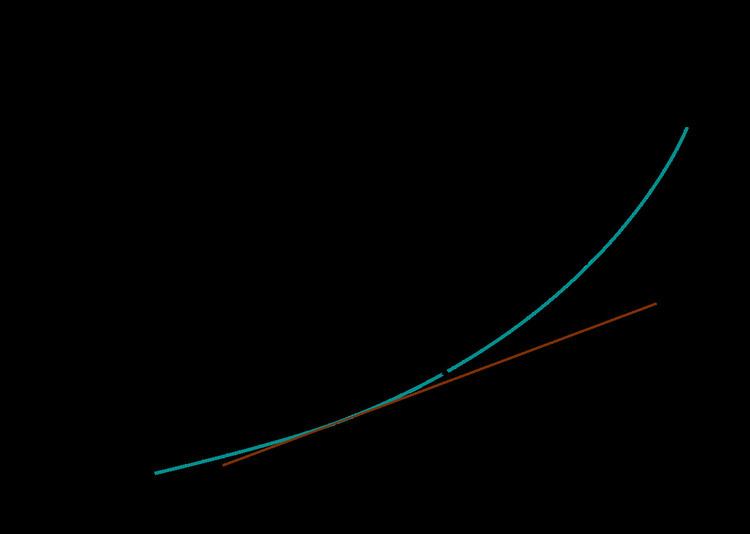
Visually, the accompanying diagram shows the tangent line of f ( x ) at x . At f ( x + h ) , where h is any small positive or negative value, f ( x + h ) is very nearly the value of the tangent line at the point ( x + h , L ( x + h ) ) .

The final equation for the linearization of a function at x = a is:

y = ( f ( a ) + f ′ ( a ) ( x − a ) )

For x = a , f ( a ) = f ( x ) . The derivative of f ( x ) is f ′ ( x ) , and the slope of f ( x ) at a is f ′ ( a ) .

Example

To find 4.001 , we can use the fact that 4 = 2 . The linearization of f ( x ) = x at x = a is y = a + 1 2 a ( x − a ) , because the function f ′ ( x ) = 1 2 x defines the slope of the function f ( x ) = x at x . Substituting in a = 4 , the linearization at 4 is y = 2 + x − 4 4 . In this case x = 4.001 , so 4.001 is approximately 2 + 4.001 − 4 4 = 2.00025 . The true value is close to 2.00024998, so the linearization approximation has a relative error of less than 1 millionth of a percent.

Linearization of a multivariable function

The equation for the linearization of a function f ( x , y ) at a point p ( a , b ) is:

f ( x , y ) ≈ f ( a , b ) + ∂ f ( x , y ) ∂ x | a , b ( x − a ) + ∂ f ( x , y ) ∂ y | a , b ( y − b )

The general equation for the linearization of a multivariable function f ( x ) at a point p is:

f ( x ) ≈ f ( p ) + ∇ f | p ⋅ ( x − p )

where x is the vector of variables, and p is the linearization point of interest .

Uses of linearization

Linearization makes it possible to use tools for studying linear systems to analyze the behavior of a nonlinear function near a given point. The linearization of a function is the first order term of its Taylor expansion around the point of interest. For a system defined by the equation

the linearized system can be written as

where x 0 is the point of interest and D F ( x 0 ) is the Jacobian of F ( x ) evaluated at x 0 .

Stability analysis

In stability analysis of autonomous systems, one can use the eigenvalues of the Jacobian matrix evaluated at a hyperbolic equilibrium point to determine the nature of that equilibrium. This is the content of linearization theorem. For time-varying systems, the linearization requires additional justification.

Microeconomics

In microeconomics, decision rules may be approximated under the state-space approach to linearization. Under this approach, the Euler equations of the utility maximization problem are linearized around the stationary steady state. A unique solution to the resulting system of dynamic equations then is found.

Optimization

In Mathematical optimization, cost functions and non-linear components within can be linearized in order to apply a linear solving method such as the Simplex algorithm. The optimized result is reached much more efficiently and is deterministic as a global optimum.