Introduction to the mathematics of general relativity

Vectors

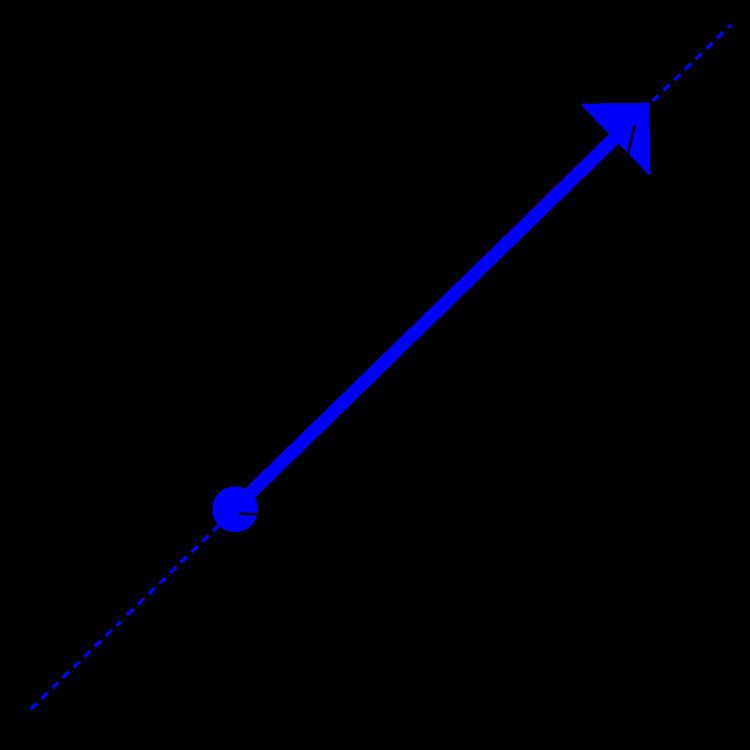
In mathematics, physics, and engineering, a Euclidean vector (sometimes called a geometric or spatial vector, or – as here – simply a vector) is a geometric object that has both a magnitude (or length) and direction. A vector is what is needed to "carry" the point A to the point B; the Latin word vector means "one who carries". The magnitude of the vector is the distance between the two points and the direction refers to the direction of displacement from A to B. Many algebraic operations on real numbers such as addition, subtraction, multiplication, and negation have close analogues for vectors, operations which obey the familiar algebraic laws of commutativity, associativity, and distributivity.

Tensors

A tensor extends the concept of a vector to additional dimensions. A scalar, that is, a simple number without a direction, would be shown on a graph as a point, a zero-dimensional object. A vector, which has a magnitude and direction, would appear on a graph as a line, which is a one-dimensional object. A tensor extends this concept to additional dimensions. A two-dimensional tensor would be called a second-order tensor. This can be viewed as a set of related vectors, moving in multiple directions on a plane.

Applications

Vectors are fundamental in the physical sciences. They can be used to represent any quantity that has both a magnitude and direction, such as velocity, the magnitude of which is speed. For example, the velocity 5 meters per second upward could be represented by the vector (0, 5) (in 2 dimensions with the positive y axis as 'up'). Another quantity represented by a vector is force, since it has a magnitude and direction. Vectors also describe many other physical quantities, such as displacement, acceleration, momentum, and angular momentum. Other physical vectors, such as the electric and magnetic field, are represented as a system of vectors at each point of a physical space; that is, a vector field.

Tensors also have extensive applications in physics:

Dimensions

In general relativity, four-dimensional vectors, or four-vectors, are required. These four dimensions are length, height, width and time. A "point" in this context would be an event, as it has both a location and a time. Similar to vectors, tensors in relativity require four dimensions. One example is the Riemann curvature tensor.

Coordinate transformation

In physics, as well as mathematics, a vector is often identified with a tuple, or list of numbers, which depend on some auxiliary coordinate system or reference frame. When the coordinates are transformed, for example by rotation or stretching, then the components of the vector also transform. The vector itself has not changed, but the reference frame has, so the components of the vector (or measurements taken with respect to the reference frame) must change to compensate.

The vector is called covariant or contravariant depending on how the transformation of the vector's components is related to the transformation of coordinates.

In Einstein notation, contravariant vectors and components of tensors are shown with superscripts, e.g. xⁱ, and covariant vectors and components of tensors with subscripts, e.g. x_i. Indices are "raised" or "lowered" by multiplication by an appropriate matrix, often the identity matrix.

Coordinate transformation is important because relativity states that there is no one correct reference point in the universe. On earth, we use dimensions like north, east, and elevation, which are used throughout the entire planet. There is no such system for space. Without a clear reference grid, it becomes more accurate to describe the four dimensions as towards/away, left/right, up/down and past/future. As an example event, take the signing of the Declaration of Independence. To a modern observer on Mount Rainier looking east, the event is ahead, to the right, below, and in the past. However, to an observer in medieval England looking north, the event is behind, to the left, neither up nor down, and in the future. The event itself has not changed, the location of the observer has.

Oblique axes

An oblique coordinate system is one in which the axes are not necessarily orthogonal to each other; that is, they meet at angles other than right angles. When using coordinate transformations as described above, the new coordinate system will often appear to have oblique axes compared to the old system.

Nontensors

A nontensor is a tensor-like quantity that behaves like a tensor in the raising and lowering of indices, but that does not transform like a tensor under a coordinate transformation. For example, Christoffel symbols cannot be tensors themselves if the coordinates don't change in a linear way.

In general relativity, one cannot describe the energy and momentum of the gravitational field by an energy–momentum tensor. Instead, one introduces objects that behave as tensors only with respect to restricted coordinate transformations. Strictly speaking, such objects are not tensors at all. A famous example of such a pseudotensor is the Landau–Lifshitz pseudotensor.

Curvilinear coordinates and curved spacetime

Curvilinear coordinates are coordinates in which the angles between axes can change from point to point. This means that rather than having a grid of straight lines, the grid instead has curvature.

A good example of this is the surface of the Earth. While maps frequently portray north, south, east and west as a simple square grid, that is not in fact the case. Instead, the longitude lines running north and south are curved and meet at the north pole. This is because the Earth is not flat, but instead round.

In general relativity, gravity has curvature effects on the four dimensions of the universe. A common analogy is placing a heavy object on a stretched out rubber sheet, causing the sheet to bend downward. This curves the coordinate system around the object, much like an object in the universe curves the coordinate system it sits in. The mathematics here are conceptually more complex than on Earth, as it results in four dimensions of curved coordinates instead of three as used to describe a curved 2D surface.

The interval in a high-dimensional space

In a Euclidean space, the separation between two points is measured by the distance between the two points. The distance is purely spatial, and is always positive. In spacetime, the separation between two events is measured by the invariant interval between the two events, which takes into account not only the spatial separation between the events, but also their temporal separation. The interval, s², between two events is defined as:

where c is the speed of light, and Δr and Δt denote differences of the space and time coordinates, respectively, between the events. The choice of signs for s² above follows the space-like convention (−+++). A notation like Δr² means (Δr)². The reason s² is called the interval and not s is that s² can be positive, zero or negative.

Spacetime intervals may be classified into three distinct types, based on whether the temporal separation (c²Δt²) or the spatial separation (Δr²) of the two events is greater: time-like, light-like or space-like.

Certain types of world lines are called geodesics of the spacetime – straight lines in the case of Minkowski space and their closest equivalent in the curved spacetime of general relativity. In the case of purely time-like paths, geodesics are (locally) the paths of greatest separation (spacetime interval) as measured along the path between two events, whereas in Euclidean space and Riemannian manifolds, geodesics are paths of shortest distance between two points. The concept of geodesics becomes central in general relativity, since geodesic motion may be thought of as "pure motion" (inertial motion) in spacetime, that is, free from any external influences.

The covariant derivative

The covariant derivative is a generalization of the directional derivative from vector calculus. As with the directional derivative, the covariant derivative is a rule, which takes as its inputs: (1) a vector, u, (along which the derivative is taken) defined at a point P, and (2) a vector field, v, defined in a neighborhood of P. The output is a vector, also at the point P. The primary difference from the usual directional derivative is that the covariant derivative must, in a certain precise sense, be independent of the manner in which it is expressed in a coordinate system.

Parallel transport

Given the covariant derivative, one can define the parallel transport of a vector v at a point P along a curve γ starting at P. For each point x of γ, the parallel transport of v at x will be a function of x, and can be written as v(x), where v(0) = v. The function v is determined by the requirement that the covariant derivative of v(x) along γ is 0. This is similar to the fact that a constant function is one whose derivative is constantly 0.

Christoffel symbols

The equation for the covariant derivative can be written down in terms of Christoffel symbols. The Christoffel symbols find frequent use in Einstein's theory of general relativity, where spacetime is represented by a curved 4-dimensional Lorentz manifold with a Levi-Civita connection. The Einstein field equations – which determine the geometry of spacetime in the presence of matter – contain the Ricci tensor, and so calculating the Christoffel symbols is essential. Once the geometry is determined, the paths of particles and light beams are calculated by solving the geodesic equations in which the Christoffel symbols explicitly appear.

Geodesics

In general relativity, a geodesic generalizes the notion of a "straight line" to curved spacetime. Importantly, the world line of a particle free from all external, non-gravitational force, is a particular type of geodesic. In other words, a freely moving or falling particle always moves along a geodesic.

In general relativity, gravity can be regarded as not a force but a consequence of a curved spacetime geometry where the source of curvature is the stress–energy tensor (representing matter, for instance). Thus, for example, the path of a planet orbiting around a star is the projection of a geodesic of the curved 4-dimensional spacetime geometry around the star onto 3-dimensional space.

A curve is a geodesic if the tangent vector of the curve at any point is equal to the parallel transport of the tangent vector of the base point.

Curvature tensor

The Riemann tensor tells us, mathematically, how much curvature there is in any given region of space. Contracting the tensor produces 3 different mathematical objects:

1. The Riemann curvature tensor: R^ρ_σμν, which gives the most information on the curvature of a space and is derived from derivatives of the metric tensor. In flat space this tensor is zero.
2. The Ricci tensor: R_σν, comes from the need in Einstein's theory for a curvature tensor with only 2 indices. It is obtained by averaging certain portions of the Riemann curvature tensor.
3. The scalar curvature: R, the simplest measure of curvature, assigns a single scalar value to each point in a space. It is obtained by averaging the Ricci tensor.

The Riemann curvature tensor can be expressed in terms of the covariant derivative.

The Einstein tensor G is a rank-2 tensor defined over pseudo-Riemannian manifolds. In index-free notation it is defined as

where R is the Ricci tensor, g is the metric tensor and R is the scalar curvature. It is used in the Einstein field equations.

Stress–energy tensor

The stress–energy tensor (sometimes stress–energy–momentum tensor or energy–momentum tensor) is a tensor quantity in physics that describes the density and flux of energy and momentum in spacetime, generalizing the stress tensor of Newtonian physics. It is an attribute of matter, radiation, and non-gravitational force fields. The stress–energy tensor is the source of the gravitational field in the Einstein field equations of general relativity, just as mass density is the source of such a field in Newtonian gravity.

Einstein equation

The Einstein field equations (EFE) or Einstein's equations are a set of 10 equations in Albert Einstein's general theory of relativity which describe the fundamental interaction of gravitation as a result of spacetime being curved by matter and energy. First published by Einstein in 1915 as a tensor equation, the EFE equate local spacetime curvature (expressed by the Einstein tensor) with the local energy and momentum within that spacetime (expressed by the stress–energy tensor).

The Einstein Field Equations can be written as

where G_μν is the Einstein tensor and T_μν is the stress–energy tensor.

This implies that the curvature of space (represented by the Einstein tensor) is directly connected to the presence of matter and energy (represented by the stress–energy tensor).

Schwarzschild solution and black holes

In Einstein's theory of general relativity, the Schwarzschild metric (also Schwarzschild vacuum or Schwarzschild solution), is a solution to the Einstein field equations which describes the gravitational field outside a spherical mass, on the assumption that the electric charge of the mass, angular momentum of the mass, and universal cosmological constant are all zero. The solution is a useful approximation for describing slowly rotating astronomical objects such as many stars and planets, including Earth and the Sun. The solution is named after Karl Schwarzschild, who first published the solution in 1916.

According to Birkhoff's theorem, the Schwarzschild metric is the most general spherically symmetric, vacuum solution of the Einstein field equations. A Schwarzschild black hole or static black hole is a black hole that has no charge or angular momentum. A Schwarzschild black hole is described by the Schwarzschild metric, and cannot be distinguished from any other Schwarzschild black hole except by its mass.