Electric susceptibility

Definition of volume susceptibility

Electric susceptibility is defined as the constant of proportionality (which may be a tensor) relating an electric field E to the induced dielectric polarization density P such that:

where

The susceptibility is related to its relative permittivity ε r by:

So in the case of a vacuum:

At the same time, the electric displacement D is related to the polarization density P by:

Molecular polarizability

A similar parameter exists to relate the magnitude of the induced dipole moment p of an individual molecule to the local electric field E that induced the dipole. This parameter is the molecular polarizability (α), and the dipole moment resulting from the local electric field E_local is given by:

This introduces a complication however, as locally the field can differ significantly from the overall applied field. We have:

where P is the polarization per unit volume, and N is the number of molecules per unit volume contributing to the polarization. Thus, if the local electric field is parallel to the ambient electric field, we have:

Thus only if the local field equals the ambient field can we write:

Otherwise, one should find a relation between the local and the macroscopic field. In some materials, the Clausius–Mossotti relation holds and reads

Ambiguity in the definition

The definition of the molecular polarizability depends on the author. In the above definition,

p and E are in SI units and the molecular polarizability α has the dimension of a volume (m³). Another definition would be to keep SI units and to integrate ε 0 into α :

In this second definition, the polarizability would have the SI unit of C.m²/V. Yet another definition exists where p and E are expressed in the cgs system and α is still defined as

Using the cgs units gives α the dimension of a volume, as in the first definition, but with a value that is 4 π lower.

Nonlinear susceptibility

In many materials the polarizability starts to saturate at high values of electric field. This saturation can be modelled by a nonlinear susceptibility. These susceptibilities are important in nonlinear optics and lead to effects such as second harmonic generation (such as used to convert infrared light into visible light, in green laser pointers).

The standard definition of nonlinear susceptibilities in SI units is via a Taylor expansion of the polarization's reaction to electric field:

(Except in ferroelectric materials, the built-in polarization is zero, P 0 = 0 .) The first susceptibility term, χ ( 1 ) , corresponds to the linear susceptibility described above. While this first term is dimensionless, the subsequent nonlinear susceptibilities χ ( n ) have units of (m/V)^n-1.

The nonlinear susceptibilities can be generalized to anisotropic materials (where each susceptibility χ ( n ) becomes an n+1-rank tensor).

Dispersion and causality

In general, a material cannot polarize instantaneously in response to an applied field, and so the more general formulation as a function of time is

That is, the polarization is a convolution of the electric field at previous times with time-dependent susceptibility given by χ e ( Δ t ) . The upper limit of this integral can be extended to infinity as well if one defines χ e ( Δ t ) = 0 for Δ t < 0 . An instantaneous response corresponds to Dirac delta function susceptibility χ e ( Δ t ) = χ e δ ( Δ t ) .

It is more convenient in a linear system to take the Fourier transform and write this relationship as a function of frequency. Due to the convolution theorem, the integral becomes a simple product,

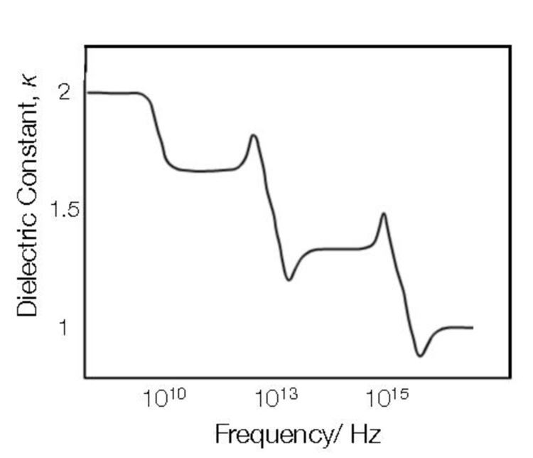
This frequency dependence of the susceptibility leads to frequency dependence of the permittivity. The shape of the susceptibility with respect to frequency characterizes the dispersion properties of the material.

Moreover, the fact that the polarization can only depend on the electric field at previous times (i.e. χ e ( Δ t ) = 0 for Δ t < 0 ), a consequence of causality, imposes Kramers–Kronig constraints on the susceptibility χ e ( 0 ) .