
 | ||
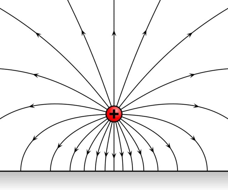
An electric field is a vector field that associates to each point in space the Coulomb force that would be experienced per unit of electric charge, by an infinitesimal test charge at that point. Electric fields are created by electric charges and can be induced by time-varying magnetic fields. The electric field combines with the magnetic field to form the electromagnetic field.
Contents
Definition
The electric field,
Its SI units are newtons per coulomb (N⋅C−1) or, equivalently, volts per metre (V⋅m−1), which in terms of SI base units are kg⋅m⋅s−3⋅A−1.
Superposition principle
Electric fields satisfy the superposition principle, because Maxwell's equations are linear. As a result, if
This principle is useful to calculate the field created by multiple point charges. If charges
Electrostatic fields
Electrostatic fields are E-fields which do not change with time, which happens when charges and currents are stationary. In that case, Coulomb's law fully describes the field.
Electric potential
If a system is static, such that magnetic fields are not time-varying, then by Faraday's law, the electric field is curl-free. In this case, one can define an electric potential, that is, a function
Parallels between electrostatic and gravitational fields
Coulomb's law, which describes the interaction of electric charges:
is similar to Newton's law of universal gravitation:
(where
This suggests similarities between the electric field E and the gravitational field g, or their associated potentials. Mass is sometimes called "gravitational charge" because of that similarity.
Electrostatic and gravitational forces both are central, conservative and obey an inverse-square law.
Uniform fields
A uniform field is one in which the electric field is constant at every point. It can be approximated by placing two conducting plates parallel to each other and maintaining a voltage (potential difference) between them; it is only an approximation because of boundary effects (near the edge of the planes, electric field is distorted because the plane does not continue). Assuming infinite planes, the magnitude of the electric field E is:
where Δϕ is the potential difference between the plates and d is the distance separating the plates. The negative sign arises as positive charges repel, so a positive charge will experience a force away from the positively charged plate, in the opposite direction to that in which the voltage increases. In micro- and nano-applications, for instance in relation to semiconductors, a typical magnitude of an electric field is in the order of 7006100000000000000♠106 V⋅m−1, achieved by applying a voltage of the order of 1 volt between conductors spaced 1 µm apart.
Electrodynamic fields
Electrodynamic fields are E-fields which do change with time, for instance when charges are in motion.
The electric field cannot be described independently of the magnetic field in that case. If A is the magnetic vector potential, defined so that
One can recover Faraday's law of induction by taking the curl of that equation
which justifies, a posteriori, the previous form for E.
Energy in the electric field
If the magnetic field B is nonzero,
The total energy per unit volume stored by the electromagnetic field is
where ε is the permittivity of the medium in which the field exists,
As E and B fields are coupled, it would be misleading to split this expression into "electric" and "magnetic" contributions. However, in the steady-state case, the fields are no longer coupled (see Maxwell's equations). It makes sense in that case to compute the electrostatic energy per unit volume:
The total energy U stored in the electric field in a given volume V is therefore
Definitive equation of vector fields
In the presence of matter, it is helpful in electromagnetism to extend the notion of the electric field into three vector fields, rather than just one:
where P is the electric polarization – the volume density of electric dipole moments, and D is the electric displacement field. Since E and P are defined separately, this equation can be used to define D. The physical interpretation of D is not as clear as E (effectively the field applied to the material) or P (induced field due to the dipoles in the material), but still serves as a convenient mathematical simplification, since Maxwell's equations can be simplified in terms of free charges and currents.
Constitutive relation
The E and D fields are related by the permittivity of the material, ε.
For linear, homogeneous, isotropic materials E and D are proportional and constant throughout the region, there is no position dependence: For inhomogeneous materials, there is a position dependence throughout the material:
For anisotropic materials the E and D fields are not parallel, and so E and D are related by the permittivity tensor (a 2nd order tensor field), in component form:
For non-linear media, E and D are not proportional. Materials can have varying extents of linearity, homogeneity and isotropy.