Infinitesimal strain theory - Alchetron, the free social encyclopedia

In continuum mechanics, the infinitesimal strain theory is a mathematical approach to the description of the deformation of a solid body in which the displacements of the material particles are assumed to be much smaller (indeed, infinitesimally smaller) than any relevant dimension of the body; so that its geometry and the constitutive properties of the material (such as density and stiffness) at each point of space can be assumed to be unchanged by the deformation.

With this assumption, the equations of continuum mechanics are considerably simplified. This approach may also be called small deformation theory, small displacement theory, or small displacement-gradient theory. It is contrasted with the finite strain theory where the opposite assumption is made.

The infinitesimal strain theory is commonly adopted in civil and mechanical engineering for the stress analysis of structures built from relatively stiff elastic materials like concrete and steel, since a common goal in the design of such structures is to minimize their deformation under typical loads.

Infinitesimal strain tensor

For infinitesimal deformations of a continuum body, in which the displacement (vector) and the displacement gradient (2nd order tensor) are small compared to unity, i.e., ∥ u ∥ ≪ 1 and ∥ ∇ u ∥ ≪ 1 , it is possible to perform a geometric linearization of any one of the (infinitely many possible) strain tensors used in finite strain theory, e.g. the Lagrangian strain tensor E , and the Eulerian strain tensor e . In such a linearization, the non-linear or second-order terms of the finite strain tensor are neglected. Thus we have

E = 1 2 ( ∇ X u + ( ∇ X u ) T + ( ∇ X u ) T ∇ X u ) ≈ 1 2 ( ∇ X u + ( ∇ X u ) T )

or

E K L = 1 2 ( ∂ U K ∂ X L + ∂ U L ∂ X K + ∂ U M ∂ X K ∂ U M ∂ X L ) ≈ 1 2 ( ∂ U K ∂ X L + ∂ U L ∂ X K )

and

e = 1 2 ( ∇ x u + ( ∇ x u ) T − ∇ x u ( ∇ x u ) T ) ≈ 1 2 ( ∇ x u + ( ∇ x u ) T )

or

e r s = 1 2 ( ∂ u r ∂ x s + ∂ u s ∂ x r − ∂ u k ∂ x r ∂ u k ∂ x s ) ≈ 1 2 ( ∂ u r ∂ x s + ∂ u s ∂ x r )

This linearization implies that the Lagrangian description and the Eulerian description are approximately the same as there is little difference in the material and spatial coordinates of a given material point in the continuum. Therefore, the material displacement gradient components and the spatial displacement gradient components are approximately equal. Thus we have

E ≈ e ≈ ε = 1 2 ( ( ∇ u ) T + ∇ u )

or E K L ≈ e r s ≈ ε i j = 1 2 ( u i , j + u j , i )

where ε i j are the components of the infinitesimal strain tensor ε , also called Cauchy's strain tensor, linear strain tensor, or small strain tensor.

ε i j = 1 2 ( u i , j + u j , i ) = [ ε 11 ε 12 ε 13 ε 21 ε 22 ε 23 ε 31 ε 32 ε 33 ] = [ ∂ u 1 ∂ x 1 1 2 ( ∂ u 1 ∂ x 2 + ∂ u 2 ∂ x 1 ) 1 2 ( ∂ u 1 ∂ x 3 + ∂ u 3 ∂ x 1 ) 1 2 ( ∂ u 2 ∂ x 1 + ∂ u 1 ∂ x 2 ) ∂ u 2 ∂ x 2 1 2 ( ∂ u 2 ∂ x 3 + ∂ u 3 ∂ x 2 ) 1 2 ( ∂ u 3 ∂ x 1 + ∂ u 1 ∂ x 3 ) 1 2 ( ∂ u 3 ∂ x 2 + ∂ u 2 ∂ x 3 ) ∂ u 3 ∂ x 3 ]

or using different notation:

[ ε x x ε x y ε x z ε y x ε y y ε y z ε z x ε z y ε z z ] = [ ∂ u x ∂ x 1 2 ( ∂ u x ∂ y + ∂ u y ∂ x ) 1 2 ( ∂ u x ∂ z + ∂ u z ∂ x ) 1 2 ( ∂ u y ∂ x + ∂ u x ∂ y ) ∂ u y ∂ y 1 2 ( ∂ u y ∂ z + ∂ u z ∂ y ) 1 2 ( ∂ u z ∂ x + ∂ u x ∂ z ) 1 2 ( ∂ u z ∂ y + ∂ u y ∂ z ) ∂ u z ∂ z ]

Furthermore, since the deformation gradient can be expressed as F = ∇ u + I where I is the second-order identity tensor, we have

ε = 1 2 ( F T + F ) − I

Also, from the general expression for the Lagrangian and Eulerian finite strain tensors we have

E ( m ) = 1 2 m ( U 2 m − I ) = 1 2 m [ ( F T F ) m − I ] ≈ 1 2 m [ { ∇ u + ( ∇ u ) T + I } m − I ] ≈ ε e ( m ) = 1 2 m ( V 2 m − I ) = 1 2 m [ ( F F T ) m − I ] ≈ ε

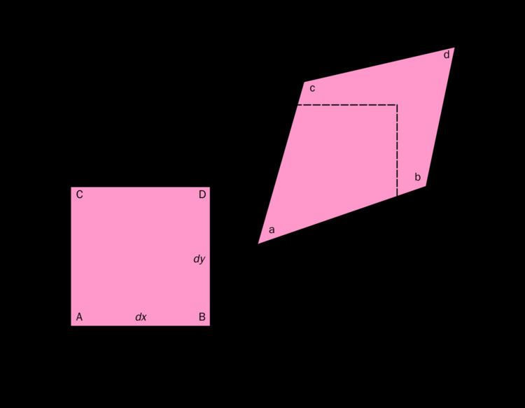
Geometric derivation of the infinitesimal strain tensor

Consider a two-dimensional deformation of an infinitesimal rectangular material element with dimensions d x by d y (Figure 1), which after deformation, takes the form of a rhombus. From the geometry of Figure 1 we have

a b ¯ = ( d x + ∂ u x ∂ x d x ) 2 + ( ∂ u y ∂ x d x ) 2 = d x 1 + 2 ∂ u x ∂ x + ( ∂ u x ∂ x ) 2 + ( ∂ u y ∂ x ) 2

For very small displacement gradients, i.e., ∥ ∇ u ∥ ≪ 1 , we have

a b ¯ ≈ d x + ∂ u x ∂ x d x

The normal strain in the x -direction of the rectangular element is defined by

ε x = a b ¯ − A B ¯ A B ¯

and knowing that A B ¯ = d x , we have

ε x = ∂ u x ∂ x

Similarly, the normal strain in the y -direction, and z -direction, becomes

ε y = ∂ u y ∂ y , ε z = ∂ u z ∂ z

The engineering shear strain, or the change in angle between two originally orthogonal material lines, in this case line A C ¯ and A B ¯ , is defined as

γ x y = α + β

From the geometry of Figure 1 we have

tan ⁡ α = ∂ u y ∂ x d x d x + ∂ u x ∂ x d x = ∂ u y ∂ x 1 + ∂ u x ∂ x , tan ⁡ β = ∂ u x ∂ y d y d y + ∂ u y ∂ y d y = ∂ u x ∂ y 1 + ∂ u y ∂ y

For small rotations, i.e. α and β are ≪ 1 we have

tan ⁡ α ≈ α , tan ⁡ β ≈ β

and, again, for small displacement gradients, we have

α = ∂ u y ∂ x , β = ∂ u x ∂ y

thus

γ x y = α + β = ∂ u y ∂ x + ∂ u x ∂ y

By interchanging x and y and u x and u y , it can be shown that γ x y = γ y x

Similarly, for the y - z and x - z planes, we have

γ y z = γ z y = ∂ u y ∂ z + ∂ u z ∂ y , γ z x = γ x z = ∂ u z ∂ x + ∂ u x ∂ z

It can be seen that the tensorial shear strain components of the infinitesimal strain tensor can then be expressed using the engineering strain definition, γ , as

[ ε x x ε x y ε x z ε y x ε y y ε y z ε z x ε z y ε z z ] = [ ε x x γ x y / 2 γ x z / 2 γ y x / 2 ε y y γ y z / 2 γ z x / 2 γ z y / 2 ε z z ]

Physical interpretation of the infinitesimal strain tensor

From finite strain theory we have

d x 2 − d X 2 = d X ⋅ 2 E ⋅ d X or ( d x ) 2 − ( d X ) 2 = 2 E K L d X K d X L

For infinitesimal strains then we have

d x 2 − d X 2 = d X ⋅ 2 ε ⋅ d X or ( d x ) 2 − ( d X ) 2 = 2 ε K L d X K d X L

Dividing by ( d X ) 2 we have

d x − d X d X d x + d X d X = 2 ε i j d X i d X d X j d X

For small deformations we assume that d x ≈ d X , thus the second term of the left hand side becomes: d x + d X d X ≈ 2 .

Then we have

d x − d X d X = ε i j N i N j = N ⋅ ε ⋅ N

where N i = d X i d X , is the unit vector in the direction of d X , and the left-hand-side expression is the normal strain e ( N ) in the direction of N . For the particular case of N in the X 1 direction, i.e. N = I 1 , we have

e ( I 1 ) = I 1 ⋅ ε ⋅ I 1 = ε 11

Similarly, for N = I 2 and N = I 3 we can find the normal strains ε 22 and ε 33 , respectively. Therefore, the diagonal elements of the infinitesimal strain tensor are the normal strains in the coordinate directions.

Strain transformation rules

If we choose an orthonormal coordinate system ( e 1 , e 2 , e 3 ) we can write the tensor in terms of components with respect to those base vectors as

ε = ∑ i = 1 3 ∑ j = 1 3 ε i j e i ⊗ e j

In matrix form,

ε _ _ = [ ε 11 ε 12 ε 13 ε 12 ε 22 ε 23 ε 13 ε 23 ε 33 ]

We can easily choose to use another orthonormal coordinate system ( e ^ 1 , e ^ 2 , e ^ 3 ) instead. In that case the components of the tensor are different, say

ε = ∑ i = 1 3 ∑ j = 1 3 ε ^ i j e ^ i ⊗ e ^ j ⟹ ε ^ _ _ = [ ε ^ 11 ε ^ 12 ε ^ 13 ε ^ 12 ε ^ 22 ε ^ 23 ε ^ 13 ε ^ 23 ε ^ 33 ]

The components of the strain in the two coordinate systems are related by

ε ^ i j = ℓ i p ℓ j q ε p q

where the Einstein summation convention for repeated indices has been used and ℓ i j = e ^ i ⋅ e j . In matrix form

ε ^ _ _ = L _ _ ε _ _ L _ _ T

or

[ ε ^ 11 ε ^ 12 ε ^ 13 ε ^ 21 ε ^ 22 ε ^ 23 ε ^ 31 ε ^ 32 ε ^ 33 ] = [ ℓ 11 ℓ 12 ℓ 13 ℓ 21 ℓ 22 ℓ 23 ℓ 31 ℓ 32 ℓ 33 ] [ ε 11 ε 12 ε 13 ε 21 ε 22 ε 23 ε 31 ε 32 ε 33 ] [ ℓ 11 ℓ 12 ℓ 13 ℓ 21 ℓ 22 ℓ 23 ℓ 31 ℓ 32 ℓ 33 ] T

Strain invariants

Certain operations on the strain tensor give the same result without regard to which orthonormal coordinate system is used to represent the components of strain. The results of these operations are called strain invariants. The most commonly used strain invariants are

I 1 = t r ( ε ) I 2 = 1 2 { t r ( ε 2 ) − [ t r ( ε ) ] 2 } I 3 = det ( ε )

In terms of components

I 1 = ε 11 + ε 22 + ε 33 I 2 = ε 12 2 + ε 23 2 + ε 31 2 − ε 11 ε 22 − ε 22 ε 33 − ε 33 ε 11 I 3 = ε 11 ( ε 22 ε 33 − ε 23 2 ) − ε 12 ( ε 12 ε 33 − ε 23 ε 31 ) + ε 13 ( ε 12 ε 23 − ε 22 ε 31 )

Principal strains

It can be shown that it is possible to find a coordinate system ( n 1 , n 2 , n 3 ) in which the components of the strain tensor are

ε _ _ = [ ε 1 0 0 0 ε 2 0 0 0 ε 3 ] ⟹ ε = ε 1 n 1 ⊗ n 1 + ε 2 n 2 ⊗ n 2 + ε 3 n 3 ⊗ n 3

The components of the strain tensor in the ( n 1 , n 2 , n 3 ) coordinate system are called the principal strains and the directions n i are called the directions of principal strain. Since there are no shear strain components in this coordinate system, the principal strains represent the maximum and minimum stretches of an elemental volume.

If we are given the components of the strain tensor in an arbitrary orthonormal coordinate system, we can find the principal strains using an eigenvalue decomposition determined by solving the system of equations

( ε _ _ − ε i I _ _ ) n i = 0 _

This system of equations is equivalent to finding the vector n i along which the stress tensor becomes a pure stretch with no shear component.

Volumetric strain

The dilatation (the relative variation of the volume) is the trace of the tensor:

δ = Δ V V 0 = ε 11 + ε 22 + ε 33

Actually, if we consider a cube with an edge length a, it is a quasi-cube after the deformation (the variations of the angles do not change the volume) with the dimensions a ⋅ ( 1 + ε 11 ) × a ⋅ ( 1 + ε 22 ) × a ⋅ ( 1 + ε 33 ) and V₀ = a³, thus

Δ V V 0 = ( 1 + ε 11 + ε 22 + ε 33 + ε 11 ⋅ ε 22 + ε 11 ⋅ ε 33 + ε 22 ⋅ ε 33 + ε 11 ⋅ ε 22 ⋅ ε 33 ) ⋅ a 3 − a 3 a 3

as we consider small deformations,

1 ≫ ε i i ≫ ε i i ⋅ ε j j ≫ ε 11 ⋅ ε 22 ⋅ ε 33

therefore the formula.

Real variation of volume (top) and the approximated one (bottom): the green drawing shows the estimated volume and the orange drawing the neglected volume

In case of pure shear, we can see that there is no change of the volume.

Strain deviator tensor

The infinitesimal strain tensor ε i j , similarly to the Cauchy stress tensor, can be expressed as the sum of two other tensors:

a mean strain tensor or volumetric strain tensor or spherical strain tensor, ε M δ i j , related to dilation or volume change; and
a deviatoric component called the strain deviator tensor, ε i j ′ , related to distortion.

ε i j = ε i j ′ + ε M δ i j

where ε M is the mean strain given by

ε M = ε k k 3 = ε 11 + ε 22 + ε 33 3 = 1 3 I 1 e

The deviatoric strain tensor can be obtained by subtracting the mean strain tensor from the infinitesimal strain tensor:

ε i j ′ = ε i j − ε k k 3 δ i j [ ε 11 ′ ε 12 ′ ε 13 ′ ε 21 ′ ε 22 ′ ε 23 ′ ε 31 ′ ε 32 ′ ε 33 ′ ] = [ ε 11 ε 12 ε 13 ε 21 ε 22 ε 23 ε 31 ε 32 ε 33 ] − [ ε M 0 0 0 ε M 0 0 0 ε M ] = [ ε 11 − ε M ε 12 ε 13 ε 21 ε 22 − ε M ε 23 ε 31 ε 32 ε 33 − ε M ]

Octahedral strains

Let ( n 1 , n 2 , n 3 ) be the directions of the three principal strains. An octahedral plane is one whose normal makes equal angles with the three principal directions. The engineering shear strain on an octahedral plane is called the octahedral shear strain and is given by

γ o c t = 2 3 ( ε 1 − ε 2 ) 2 + ( ε 2 − ε 3 ) 2 + ( ε 3 − ε 1 ) 2

where ε 1 , ε 2 , ε 3 are the principal strains.

The normal strain on an octahedral plane is given by

ε o c t = 1 3 ( ε 1 + ε 2 + ε 3 )

Equivalent strain

A scalar quantity called the equivalent strain, or the von Mises equivalent strain, is often used to describe the state of strain in solids. Several definitions of equivalent strain can be found in the literature. A definition that is commonly used in the literature on plasticity is

ε e q = 2 3 ε d e v : ε d e v = 2 3 ε i j d e v ε i j d e v ; ε d e v = ε − 1 3 t r ( ε ) I

This quantity is work conjugate to the equivalent stress defined as

σ e q = 3 2 σ d e v : σ d e v

Compatibility equations

For prescribed strain components ε i j the strain tensor equation u i , j + u j , i = 2 ε i j represents a system of six differential equations for the determination of three displacements components u i , giving an over-determined system. Thus, a solution does not generally exist for an arbitrary choice of strain components. Therefore, some restrictions, named compatibility equations, are imposed upon the strain components. With the addition of the three compatibility equations the number of independent equations are reduced to three, matching the number of unknown displacement components. These constraints on the strain tensor were discovered by Saint-Venant, and are called the "Saint Venant compatibility equations".

The compatibility functions serve to assure a single-valued continuous displacement function u i . If the elastic medium is visualised as a set of infinitesimal cubes in the unstrained state, after the medium is strained, an arbitrary strain tensor may not yield a situation in which the distorted cubes still fit together without overlapping.

In index notation, the compatibility equations are expressed as

ε i j , k m + ε k m , i j − ε i k , j m − ε j m , i k = 0

Plane strain

In real engineering components, stress (and strain) are 3-D tensors but in prismatic structures such as a long metal billet, the length of the structure is much greater than the other two dimensions. The strains associated with length, i.e., the normal strain ε 33 and the shear strains ε 13 and ε 23 (if the length is the 3-direction) are constrained by nearby material and are small compared to the cross-sectional strains. Plane strain is then an acceptable approximation. The strain tensor for plane strain is written as:

ε _ _ = [ ε 11 ε 12 0 ε 21 ε 22 0 0 0 0 ]

in which the double underline indicates a second order tensor. This strain state is called plane strain. The corresponding stress tensor is:

σ _ _ = [ σ 11 σ 12 0 σ 21 σ 22 0 0 0 σ 33 ]

in which the non-zero σ 33 is needed to maintain the constraint ϵ 33 = 0 . This stress term can be temporarily removed from the analysis to leave only the in-plane terms, effectively reducing the 3-D problem to a much simpler 2-D problem.

Antiplane strain

Antiplane strain is another special state of strain that can occur in a body, for instance in a region close to a screw dislocation. The strain tensor for antiplane strain is given by

ε _ _ = [ 0 0 ε 13 0 0 ε 23 ε 13 ε 23 0 ]

Infinitesimal rotation tensor

The infinitesimal strain tensor is defined as

ε = 1 2 [ ∇ u + ( ∇ u ) T ]

Therefore the displacement gradient can be expressed as

∇ u = ε + ω

where

ω := 1 2 [ ∇ u − ( ∇ u ) T ]

The quantity ω is the infinitesimal rotation tensor. This tensor is skew symmetric. For infinitesimal deformations the scalar components of ω satisfy the condition | ω i j | ≪ 1 . Note that the displacement gradient is small only if both the strain tensor and the rotation tensor are infinitesimal.

The axial vector

A skew symmetric second-order tensor has three independent scalar components. These three components are used to define an axial vector, w , as follows

ω i j = − ϵ i j k w k ; w i = − 1 2 ϵ i j k ω j k

where ϵ i j k is the permutation symbol. In matrix form

ω _ _ = [ 0 − w 3 w 2 w 3 0 − w 1 − w 2 w 1 0 ] ; w _ = [ w 1 w 2 w 3 ]

The axial vector is also called the infinitesimal rotation vector. The rotation vector is related to the displacement gradient by the relation

w = 1 2 ∇ × u

In index notation

w i = 1 2 ϵ i j k u k , j

If ∥ ω ∥ ≪ 1 and ε = 0 then the material undergoes an approximate rigid body rotation of magnitude | w | around the vector w .

Relation between the strain tensor and the rotation vector

Given a continuous, single-valued displacement field u and the corresponding infinitesimal strain tensor ε , we have (see Tensor derivative (continuum mechanics))

∇ × ε = e i j k ε l j , i e k ⊗ e l = 1 2 e i j k [ u l , j i + u j , l i ] e k ⊗ e l

Since a change in the order of differentiation does not change the result, u l , j i = u l , i j . Therefore

e i j k u l , j i = ( e 12 k + e 21 k ) u l , 12 + ( e 13 k + e 31 k ) u l , 13 + ( e 23 k + e 32 k ) u l , 32 = 0

Also

1 2 e i j k u j , l i = ( 1 2 e i j k u j , i ) , l = ( 1 2 e k i j u j , i ) , l = w k , l

Hence

∇ × ε = w k , l e k ⊗ e l = ∇ w

Relation between rotation tensor and rotation vector

From an important identity regarding the curl of a tensor we know that for a continuous, single-valued displacement field u ,

∇ × ( ∇ u ) = 0 .

Since ∇ u = ε + ω we have ∇ × ω = − ∇ × ε = − ∇ w .

Strain tensor in cylindrical coordinates

In cylindrical polar coordinates ( r , θ , z ), the displacement vector can be written as

u = u r e r + u θ e θ + u z e z

The components of the strain tensor in a cylindrical coordinate system are given by

ε r r = ∂ u r ∂ r ε θ θ = 1 r ( ∂ u θ ∂ θ + u r ) ε z z = ∂ u z ∂ z ε r θ = 1 2 ( 1 r ∂ u r ∂ θ + ∂ u θ ∂ r − u θ r ) ε θ z = 1 2 ( ∂ u θ ∂ z + 1 r ∂ u z ∂ θ ) ε z r = 1 2 ( ∂ u r ∂ z + ∂ u z ∂ r )

Strain tensor in spherical coordinates

In spherical coordinates ( r , θ , ϕ ), the displacement vector can be written as

u = u r e r + u θ e θ + u ϕ e ϕ

The components of the strain tensor in a spherical coordinate system are given by

ε r r = ∂ u r ∂ r ε θ θ = 1 r ( ∂ u θ ∂ θ + u r ) ε ϕ ϕ = 1 r sin ⁡ θ ( ∂ u ϕ ∂ ϕ + u r sin ⁡ θ + u θ cos ⁡ θ ) ε r θ = 1 2 ( 1 r ∂ u r ∂ θ + ∂ u θ ∂ r − u θ r ) ε θ ϕ = 1 2 r ( 1 sin ⁡ θ ∂ u θ ∂ ϕ + ∂ u ϕ ∂ θ − u ϕ cot ⁡ θ ) ε ϕ r = 1 2 ( 1 r sin ⁡ θ ∂ u r ∂ ϕ + ∂ u ϕ ∂ r − u ϕ r )

References

Infinitesimal strain theory Wikipedia

(Text) CC BY-SA

Contents