Cauchy stress tensor

Euler–Cauchy stress principle – stress vector

The Euler–Cauchy stress principle states that upon any surface (real or imaginary) that divides the body, the action of one part of the body on the other is equivalent (equipollent) to the system of distributed forces and couples on the surface dividing the body, and it is represented by a field T ( n ) , called the stress vector, defined on the surface S and assumed to depend continuously on the surface's unit vector n .

To formulate the Euler–Cauchy stress principle, consider an imaginary surface S passing through an internal material point P dividing the continuous body into two segments, as seen in Figure 2.1a or 2.1b (one may use either the cutting plane diagram or the diagram with the arbitrary volume inside the continuum enclosed by the surface S ).

Following the classical dynamics of Newton and Euler, the motion of a material body is produced by the action of externally applied forces which are assumed to be of two kinds: surface forces F and body forces b . Thus, the total force F applied to a body or to a portion of the body can be expressed as:

F = b + F

Only surface forces will be discussed in this article as they are relevant to the Cauchy stress tensor.

When the body is subjected to external surface forces or contact forces F , following Euler's equations of motion, internal contact forces and moments are transmitted from point to point in the body, and from one segment to the other through the dividing surface S , due to the mechanical contact of one portion of the continuum onto the other (Figure 2.1a and 2.1b). On an element of area Δ S containing P , with normal vector n , the force distribution is equipollent to a contact force Δ F exerted at point P and surface moment Δ M . In particular, the contact force is given by

Δ F = T ( n ) Δ S

where T ( n ) is the mean surface traction.

Cauchy’s stress principle asserts that as Δ S becomes very small and tends to zero the ratio Δ F / Δ S becomes d F / d S and the couple stress vector Δ M vanishes. In specific fields of continuum mechanics the couple stress is assumed not to vanish; however, classical branches of continuum mechanics address non-polar materials which do not consider couple stresses and body moments.

The resultant vector d F / d S is defined as the surface traction, also called stress vector, traction, or traction vector. given by T ( n ) = T i ( n ) e i at the point P associated with a plane with a normal vector n :

T i ( n ) = lim Δ S → 0 Δ F i Δ S = d F i d S .

This equation means that the stress vector depends on its location in the body and the orientation of the plane on which it is acting.

This implies that the balancing action of internal contact forces generates a contact force density or Cauchy traction field T ( n , x , t ) that represents a distribution of internal contact forces throughout the volume of the body in a particular configuration of the body at a given time t . It is not a vector field because it depends not only on the position x of a particular material point, but also on the local orientation of the surface element as defined by its normal vector n .

Depending on the orientation of the plane under consideration, the stress vector may not necessarily be perpendicular to that plane, i.e. parallel to n , and can be resolved into two components (Figure 2.1c):

one normal to the plane, called normal stress

σ n = lim Δ S → 0 Δ F n Δ S = d F n d S , where d F n is the normal component of the force d F to the differential area d S

and the other parallel to this plane, called the shear stress

τ = lim Δ S → 0 Δ F s Δ S = d F s d S , where d F s is the tangential component of the force d F to the differential surface area d S . The shear stress can be further decomposed into two mutually perpendicular vectors.

Cauchy’s postulate

According to the Cauchy Postulate, the stress vector T ( n ) remains unchanged for all surfaces passing through the point P and having the same normal vector n at P , i.e., having a common tangent at P . This means that the stress vector is a function of the normal vector n only, and is not influenced by the curvature of the internal surfaces.

Cauchy’s fundamental lemma

A consequence of Cauchy’s postulate is Cauchy’s Fundamental Lemma, also called the Cauchy reciprocal theorem, which states that the stress vectors acting on opposite sides of the same surface are equal in magnitude and opposite in direction. Cauchy’s fundamental lemma is equivalent to Newton's third law of motion of action and reaction, and is expressed as

− T ( n ) = T ( − n ) .

Cauchy’s stress theorem—stress tensor

The state of stress at a point in the body is then defined by all the stress vectors T⁽ⁿ⁾ associated with all planes (infinite in number) that pass through that point. However, according to Cauchy’s fundamental theorem, also called Cauchy’s stress theorem, merely by knowing the stress vectors on three mutually perpendicular planes, the stress vector on any other plane passing through that point can be found through coordinate transformation equations.

Cauchy’s stress theorem states that there exists a second-order tensor field σ(x, t), called the Cauchy stress tensor, independent of n, such that T is a linear function of n:

T ( n ) = n ⋅ σ or T j ( n ) = σ i j n i .

This equation implies that the stress vector T⁽ⁿ⁾ at any point P in a continuum associated with a plane with normal unit vector n can be expressed as a function of the stress vectors on the planes perpendicular to the coordinate axes, i.e. in terms of the components σ_ij of the stress tensor σ.

To prove this expression, consider a tetrahedron with three faces oriented in the coordinate planes, and with an infinitesimal area dA oriented in an arbitrary direction specified by a normal unit vector n (Figure 2.2). The tetrahedron is formed by slicing the infinitesimal element along an arbitrary plane n. The stress vector on this plane is denoted by T⁽ⁿ⁾. The stress vectors acting on the faces of the tetrahedron are denoted as T^(e₁), T^(e₂), and T^(e₃), and are by definition the components σ_ij of the stress tensor σ. This tetrahedron is sometimes called the Cauchy tetrahedron. The equilibrium of forces, i.e. Euler’s first law of motion (Newton’s second law of motion), gives:

T ( n ) d A − T ( e 1 ) d A 1 − T ( e 2 ) d A 2 − T ( e 3 ) d A 3 = ρ ( h 3 d A ) a ,

where the right-hand-side represents the product of the mass enclosed by the tetrahedron and its acceleration: ρ is the density, a is the acceleration, and h is the height of the tetrahedron, considering the plane n as the base. The area of the faces of the tetrahedron perpendicular to the axes can be found by projecting dA into each face (using the dot product):

d A 1 = ( n ⋅ e 1 ) d A = n 1 d A , d A 2 = ( n ⋅ e 2 ) d A = n 2 d A , d A 3 = ( n ⋅ e 3 ) d A = n 3 d A ,

and then substituting into the equation to cancel out dA:

T ( n ) − T ( e 1 ) n 1 − T ( e 2 ) n 2 − T ( e 3 ) n 3 = ρ ( h 3 ) a .

To consider the limiting case as the tetrahedron shrinks to a point, h must go to 0 (intuitively, the plane n is translated along n toward O). As a result, the right-hand-side of the equation approaches 0, so

T ( n ) = T ( e 1 ) n 1 + T ( e 2 ) n 2 + T ( e 3 ) n 3 .

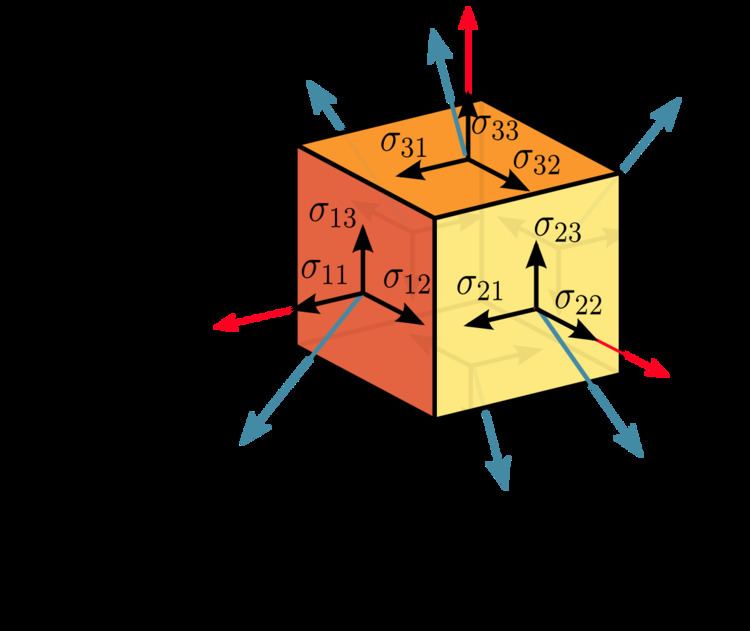
Assuming a material element (Figure 2.3) with planes perpendicular to the coordinate axes of a Cartesian coordinate system, the stress vectors associated with each of the element planes, i.e. T^(e₁), T^(e₂), and T^(e₃) can be decomposed into a normal component and two shear components, i.e. components in the direction of the three coordinate axes. For the particular case of a surface with normal unit vector oriented in the direction of the x₁-axis, denote the normal stress by σ₁₁, and the two shear stresses as σ₁₂ and σ₁₃:

T ( e 1 ) = T 1 ( e 1 ) e 1 + T 2 ( e 1 ) e 2 + T 3 ( e 1 ) e 3 = σ 11 e 1 + σ 12 e 2 + σ 13 e 3 , T ( e 2 ) = T 1 ( e 2 ) e 1 + T 2 ( e 2 ) e 2 + T 3 ( e 2 ) e 3 = σ 21 e 1 + σ 22 e 2 + σ 23 e 3 , T ( e 3 ) = T 1 ( e 3 ) e 1 + T 2 ( e 3 ) e 2 + T 3 ( e 3 ) e 3 = σ 31 e 1 + σ 32 e 2 + σ 33 e 3 ,

In index notation this is

T ( e i ) = T j ( e i ) e j = σ i j e j .

The nine components σ_ij of the stress vectors are the components of a second-order Cartesian tensor called the Cauchy stress tensor, which completely defines the state of stress at a point and is given by

σ = σ i j = [ T ( e 1 ) T ( e 2 ) T ( e 3 ) ] = [ σ 11 σ 12 σ 13 σ 21 σ 22 σ 23 σ 31 σ 32 σ 33 ] ≡ [ σ x x σ x y σ x z σ y x σ y y σ y z σ z x σ z y σ z z ] ≡ [ σ x τ x y τ x z τ y x σ y τ y z τ z x τ z y σ z ] ,

where σ₁₁, σ₂₂, and σ₃₃ are normal stresses, and σ₁₂, σ₁₃, σ₂₁, σ₂₃, σ₃₁, and σ₃₂ are shear stresses. The first index i indicates that the stress acts on a plane normal to the x_i-axis, and the second index j denotes the direction in which the stress acts. A stress component is positive if it acts in the positive direction of the coordinate axes, and if the plane where it acts has an outward normal vector pointing in the positive coordinate direction.

Thus, using the components of the stress tensor

T ( n ) = T ( e 1 ) n 1 + T ( e 2 ) n 2 + T ( e 3 ) n 3 = ∑ i = 1 3 T ( e i ) n i = ( σ i j e j ) n i = σ i j n i e j

or, equivalently,

T j ( n ) = σ i j n i .

Alternatively, in matrix form we have

[ T 1 ( n ) T 2 ( n ) T 3 ( n ) ] = [ n 1 n 2 n 3 ] ⋅ [ σ 11 σ 12 σ 13 σ 21 σ 22 σ 23 σ 31 σ 32 σ 33 ] .

The Voigt notation representation of the Cauchy stress tensor takes advantage of the symmetry of the stress tensor to express the stress as a six-dimensional vector of the form:

σ = [ σ 1 σ 2 σ 3 σ 4 σ 5 σ 6 ] T ≡ [ σ 11 σ 22 σ 33 σ 23 σ 13 σ 12 ] T .

The Voigt notation is used extensively in representing stress–strain relations in solid mechanics and for computational efficiency in numerical structural mechanics software.

Transformation rule of the stress tensor

It can be shown that the stress tensor is a contravariant second order tensor, which is a statement of how it transforms under a change of the coordinate system. From an x_i-system to an x_i' -system, the components σ_ij in the initial system are transformed into the components σ_ij' in the new system according to the tensor transformation rule (Figure 2.4):

σ i j ′ = a i m a j n σ m n or σ ′ = A σ A T ,

where A is a rotation matrix with components a_ij. In matrix form this is

[ σ 11 ′ σ 12 ′ σ 13 ′ σ 21 ′ σ 22 ′ σ 23 ′ σ 31 ′ σ 32 ′ σ 33 ′ ] = [ a 11 a 12 a 13 a 21 a 22 a 23 a 31 a 32 a 33 ] [ σ 11 σ 12 σ 13 σ 21 σ 22 σ 23 σ 31 σ 32 σ 33 ] [ a 11 a 21 a 31 a 12 a 22 a 32 a 13 a 23 a 33 ] .

Expanding the matrix operation, and simplifying terms using the symmetry of the stress tensor, gives

σ 11 ′ = a 11 2 σ 11 + a 12 2 σ 22 + a 13 2 σ 33 + 2 a 11 a 12 σ 12 + 2 a 11 a 13 σ 13 + 2 a 12 a 13 σ 23 , σ 22 ′ = a 21 2 σ 11 + a 22 2 σ 22 + a 23 2 σ 33 + 2 a 21 a 22 σ 12 + 2 a 21 a 23 σ 13 + 2 a 22 a 23 σ 23 , σ 33 ′ = a 31 2 σ 11 + a 32 2 σ 22 + a 33 2 σ 33 + 2 a 31 a 32 σ 12 + 2 a 31 a 33 σ 13 + 2 a 32 a 33 σ 23 , σ 12 ′ = a 11 a 21 σ 11 + a 12 a 22 σ 22 + a 13 a 23 σ 33 + ( a 11 a 22 + a 12 a 21 ) σ 12 + ( a 12 a 23 + a 13 a 22 ) σ 23 + ( a 11 a 23 + a 13 a 21 ) σ 13 , σ 23 ′ = a 21 a 31 σ 11 + a 22 a 32 σ 22 + a 23 a 33 σ 33 + ( a 21 a 32 + a 22 a 31 ) σ 12 + ( a 22 a 33 + a 23 a 32 ) σ 23 + ( a 21 a 33 + a 23 a 31 ) σ 13 , σ 13 ′ = a 11 a 31 σ 11 + a 12 a 32 σ 22 + a 13 a 33 σ 33 + ( a 11 a 32 + a 12 a 31 ) σ 12 + ( a 12 a 33 + a 13 a 32 ) σ 23 + ( a 11 a 33 + a 13 a 31 ) σ 13 .

The Mohr circle for stress is a graphical representation of this transformation of stresses.

Normal and shear stresses

The magnitude of the normal stress component σ_n of any stress vector T⁽ⁿ⁾ acting on an arbitrary plane with normal unit vector n at a given point, in terms of the components σ_ij of the stress tensor σ, is the dot product of the stress vector and the normal unit vector:

σ n = T ( n ) ⋅ n = T i ( n ) n i = σ i j n i n j .

The magnitude of the shear stress component τ_n, acting orthogonal to the vector n, can then be found using the Pythagorean theorem:

τ n = ( T ( n ) ) 2 − σ n 2 = T i ( n ) T i ( n ) − σ n 2 ,

where

( T ( n ) ) 2 = T i ( n ) T i ( n ) = ( σ i j n j ) ( σ i k n k ) = σ i j σ i k n j n k .

Cauchy's first law of motion

According to the principle of conservation of linear momentum, if the continuum body is in static equilibrium it can be demonstrated that the components of the Cauchy stress tensor in every material point in the body satisfy the equilibrium equations.

σ j i , j + F i = 0

For example, for a hydrostatic fluid in equilibrium conditions, the stress tensor takes on the form:

σ i j = − p δ i j ,

where p is the hydrostatic pressure, and δ i j   is the kronecker delta.

Cauchy's second law of motion

According to the principle of conservation of angular momentum, equilibrium requires that the summation of moments with respect to an arbitrary point is zero, which leads to the conclusion that the stress tensor is symmetric, thus having only six independent stress components, instead of the original nine:

σ i j = σ j i

However, in the presence of couple-stresses, i.e. moments per unit volume, the stress tensor is non-symmetric. This also is the case when the Knudsen number is close to one, K n → 1 , or the continuum is a non-Newtonian fluid, which can lead to rotationally non-invariant fluids, such as polymers.

Principal stresses and stress invariants

At every point in a stressed body there are at least three planes, called principal planes, with normal vectors n , called principal directions, where the corresponding stress vector is perpendicular to the plane, i.e., parallel or in the same direction as the normal vector n , and where there are no normal shear stresses τ n . The three stresses normal to these principal planes are called principal stresses.

The components σ i j of the stress tensor depend on the orientation of the coordinate system at the point under consideration. However, the stress tensor itself is a physical quantity and as such, it is independent of the coordinate system chosen to represent it. There are certain invariants associated with every tensor which are also independent of the coordinate system. For example, a vector is a simple tensor of rank one. In three dimensions, it has three components. The value of these components will depend on the coordinate system chosen to represent the vector, but the magnitude of the vector is a physical quantity (a scalar) and is independent of the Cartesian coordinate system chosen to represent the vector. Similarly, every second rank tensor (such as the stress and the strain tensors) has three independent invariant quantities associated with it. One set of such invariants are the principal stresses of the stress tensor, which are just the eigenvalues of the stress tensor. Their direction vectors are the principal directions or eigenvectors.

A stress vector parallel to the normal unit vector n is given by:

T ( n ) = λ n = σ n n

where λ is a constant of proportionality, and in this particular case corresponds to the magnitudes σ n of the normal stress vectors or principal stresses.

Knowing that T i ( n ) = σ i j n j and n i = δ i j n j , we have

T i ( n ) = λ n i σ i j n j = λ n i σ i j n j − λ n i = 0 ( σ i j − λ δ i j ) n j = 0

This is a homogeneous system, i.e. equal to zero, of three linear equations where n j are the unknowns. To obtain a nontrivial (non-zero) solution for n j , the determinant matrix of the coefficients must be equal to zero, i.e. the system is singular. Thus,

| σ i j − λ δ i j | = | σ 11 − λ σ 12 σ 13 σ 21 σ 22 − λ σ 23 σ 31 σ 32 σ 33 − λ | = 0

Expanding the determinant leads to the characteristic equation

| σ i j − λ δ i j | = − λ 3 + I 1 λ 2 − I 2 λ + I 3 = 0

where

I 1 = σ 11 + σ 22 + σ 33 = σ k k = tr ( σ ) I 2 = | σ 22 σ 23 σ 32 σ 33 | + | σ 11 σ 13 σ 31 σ 33 | + | σ 11 σ 12 σ 21 σ 22 | = σ 11 σ 22 + σ 22 σ 33 + σ 11 σ 33 − σ 12 2 − σ 23 2 − σ 31 2 = 1 2 ( σ i i σ j j − σ i j σ j i ) I 3 = det ( σ i j ) = det ( σ ) = σ 11 σ 22 σ 33 + 2 σ 12 σ 23 σ 31 − σ 12 2 σ 33 − σ 23 2 σ 11 − σ 31 2 σ 22

The characteristic equation has three real roots λ i , i.e. not imaginary due to the symmetry of the stress tensor. The σ 1 = max ( λ 1 , λ 2 , λ 3 ) , σ 3 = min ( λ 1 , λ 2 , λ 3 ) and σ 2 = I 1 − σ 1 − σ 3 , are the principal stresses, functions of the eigenvalues λ i . The eigenvalues are the roots of the characteristic polynomial. The principal stresses are unique for a given stress tensor. Therefore, from the characteristic equation, the coefficients I 1 , I 2 and I 3 , called the first, second, and third stress invariants, respectively, always have the same value regardless of the coordinate system's orientation.

For each eigenvalue, there is a non-trivial solution for n j in the equation ( σ i j − λ δ i j ) n j = 0 . These solutions are the principal directions or eigenvectors defining the plane where the principal stresses act. The principal stresses and principal directions characterize the stress at a point and are independent of the orientation.

A coordinate system with axes oriented to the principal directions implies that the normal stresses are the principal stresses and the stress tensor is represented by a diagonal matrix:

σ i j = [ σ 1 0 0 0 σ 2 0 0 0 σ 3 ]

The principal stresses can be combined to form the stress invariants, I 1 , I 2 , and I 3 . The first and third invariant are the trace and determinant respectively, of the stress tensor. Thus,

I 1 = σ 1 + σ 2 + σ 3 I 2 = σ 1 σ 2 + σ 2 σ 3 + σ 3 σ 1 I 3 = σ 1 σ 2 σ 3

Because of its simplicity, the principal coordinate system is often useful when considering the state of the elastic medium at a particular point. Principal stresses are often expressed in the following equation for evaluating stresses in the x and y directions or axial and bending stresses on a part. The principal normal stresses can then be used to calculate the von Mises stress and ultimately the safety factor and margin of safety.

σ 1 , σ 2 = σ x + σ y 2 ± ( σ x − σ y 2 ) 2 + τ x y 2

Using just the part of the equation under the square root is equal to the maximum and minimum shear stress for plus and minus. This is shown as:

τ m a x , τ m i n = ± ( σ x − σ y 2 ) 2 + τ x y 2

Maximum and minimum shear stresses

The maximum shear stress or maximum principal shear stress is equal to one-half the difference between the largest and smallest principal stresses, and acts on the plane that bisects the angle between the directions of the largest and smallest principal stresses, i.e. the plane of the maximum shear stress is oriented 45 ∘ from the principal stress planes. The maximum shear stress is expressed as

τ max = 1 2 | σ max − σ min |

Assuming σ 1 ≥ σ 2 ≥ σ 3 then

τ max = 1 2 | σ 1 − σ 3 |

When the stress tensor is non zero the normal stress component acting on the plane for the maximum shear stress is non-zero and it is equal to

σ n = 1 2 ( σ 1 + σ 3 )

Stress deviator tensor

The stress tensor σ i j can be expressed as the sum of two other stress tensors:

1. a mean hydrostatic stress tensor or volumetric stress tensor or mean normal stress tensor, π δ i j , which tends to change the volume of the stressed body; and
2. a deviatoric component called the stress deviator tensor, s i j , which tends to distort it.

So:

σ i j = s i j + π δ i j ,

where π is the mean stress given by

π = σ k k 3 = σ 11 + σ 22 + σ 33 3 = 1 3 I 1 .

Pressure ( p ) is generally defined as negative one-third the trace of the stress tensor minus any stress the divergence of the velocity contributes with, i.e.

p = λ ∇ ⋅ u → − π = λ ∂ u k ∂ x k − π = ∑ k λ ∂ u k ∂ x k − π ,

where λ is a proportionality constant, ∇ is the divergence operator, x k is the k:th Cartesian coordinate, u → is the velocity and u k is the k:th Cartesian component of u → .

The deviatoric stress tensor can be obtained by subtracting the hydrostatic stress tensor from the Cauchy stress tensor:

  s i j = σ i j − σ k k 3 δ i j , [ s 11 s 12 s 13 s 21 s 22 s 23 s 31 s 32 s 33 ] = [ σ 11 σ 12 σ 13 σ 21 σ 22 σ 23 σ 31 σ 32 σ 33 ] − [ π 0 0 0 π 0 0 0 π ] = [ σ 11 − π σ 12 σ 13 σ 21 σ 22 − π σ 23 σ 31 σ 32 σ 33 − π ] .

Invariants of the stress deviator tensor

As it is a second order tensor, the stress deviator tensor also has a set of invariants, which can be obtained using the same procedure used to calculate the invariants of the stress tensor. It can be shown that the principal directions of the stress deviator tensor s i j are the same as the principal directions of the stress tensor σ i j . Thus, the characteristic equation is

| s i j − λ δ i j | = − λ 3 + J 1 λ 2 − J 2 λ + J 3 = 0 ,

where J 1 , J 2 and J 3 are the first, second, and third deviatoric stress invariants, respectively. Their values are the same (invariant) regardless of the orientation of the coordinate system chosen. These deviatoric stress invariants can be expressed as a function of the components of s i j or its principal values s 1 , s 2 , and s 3 , or alternatively, as a function of σ i j or its principal values σ 1 , σ 2 , and σ 3 . Thus,

J 1 = s k k = 0 , J 2 = 1 2 s i j s j i = 1 2 tr ( s 2 ) = 1 2 ( s 1 2 + s 2 2 + s 3 2 ) = 1 6 [ ( σ 11 − σ 22 ) 2 + ( σ 22 − σ 33 ) 2 + ( σ 33 − σ 11 ) 2 ] + σ 12 2 + σ 23 2 + σ 31 2 = 1 6 [ ( σ 1 − σ 2 ) 2 + ( σ 2 − σ 3 ) 2 + ( σ 3 − σ 1 ) 2 ] = 1 3 I 1 2 − I 2 = 1 2 [ tr ( σ 2 ) − 1 3 tr ( σ ) 2 ] , J 3 = det ( s i j ) = 1 3 s i j s j k s k i = 1 3 tr ( s 3 ) = 1 3 ( s 1 3 + s 2 3 + s 3 3 ) = s 1 s 2 s 3 = 2 27 I 1 3 − 1 3 I 1 I 2 + I 3 = 1 3 [ tr ( σ 3 ) − tr ( σ 2 ) tr ( σ ) + 2 9 tr ( σ ) 3 ] .

Because s k k = 0 , the stress deviator tensor is in a state of pure shear.

A quantity called the equivalent stress or von Mises stress is commonly used in solid mechanics. The equivalent stress is defined as

σ e = 3   J 2 = 1 2   [ ( σ 1 − σ 2 ) 2 + ( σ 2 − σ 3 ) 2 + ( σ 3 − σ 1 ) 2 ] .

Octahedral stresses

Considering the principal directions as the coordinate axes, a plane whose normal vector makes equal angles with each of the principal axes (i.e. having direction cosines equal to | 1 / 3 | ) is called an octahedral plane. There are a total of eight octahedral planes (Figure 6). The normal and shear components of the stress tensor on these planes are called octahedral normal stress σ o c t and octahedral shear stress τ o c t , respectively.

Knowing that the stress tensor of point O (Figure 6) in the principal axes is

σ i j = [ σ 1 0 0 0 σ 2 0 0 0 σ 3 ]

the stress vector on an octahedral plane is then given by:

T o c t ( n ) = σ i j n i e j = σ 1 n 1 e 1 + σ 2 n 2 e 2 + σ 3 n 3 e 3 = 1 3 ( σ 1 e 1 + σ 2 e 2 + σ 3 e 3 )

The normal component of the stress vector at point O associated with the octahedral plane is

σ o c t = T i ( n ) n i = σ i j n i n j = σ 1 n 1 n 1 + σ 2 n 2 n 2 + σ 3 n 3 n 3 = 1 3 ( σ 1 + σ 2 + σ 3 ) = 1 3 I 1

which is the mean normal stress or hydrostatic stress. This value is the same in all eight octahedral planes. The shear stress on the octahedral plane is then

τ o c t = T i ( n ) T i ( n ) − σ n 2 = [ 1 3 ( σ 1 2 + σ 2 2 + σ 3 2 ) − 1 9 ( σ 1 + σ 2 + σ 3 ) 2 ] 1 / 2 = 1 3 [ ( σ 1 − σ 2 ) 2 + ( σ 2 − σ 3 ) 2 + ( σ 3 − σ 1 ) 2 ] 1 / 2 = 1 3 2 I 1 2 − 6 I 2 = 2 3 J 2