Linear canonical transformation - Alchetron, the free social encyclopedia

In Hamiltonian mechanics, the linear canonical transformation (LCT) is a family of integral transforms that generalizes many classical transforms. It has 4 parameters and 1 constraint, so it is a 3-dimensional family, and can be visualized as the action of the special linear group SL₂(R) on the time–frequency plane (domain).

The LCT generalizes the Fourier, fractional Fourier, Laplace, Gauss–Weierstrass, Bargmann and the Fresnel transforms as particular cases. The name "linear canonical transformation" is from canonical transformation, a map that preserves the symplectic structure, as SL₂(R) can also be interpreted as the symplectic group Sp₂, and thus LCTs are the linear maps of the time–frequency domain which preserve the symplectic form.

Definition

The LCT can be represented in several ways; most easily, it can be parameterized by a 2×2 matrix with determinant 1, i.e., an element of the special linear group SL₂(R). Then for any such matrix ( a b c d ) , with ad − bc = 1, the corresponding integral transform from a function x ( t ) to X ( u ) is defined as

Special cases

Many classical transforms are special cases of the linear canonical transform:

The Fourier transform corresponds to rotation by 90°, represented by the matrix:

The fractional Fourier transform corresponds to rotation by an arbitrary angle; they are the elliptic elements of SL₂(R), represented by the matrices:

The Fresnel transform corresponds to shearing, and are a family of parabolic elements, represented by the matrices:

where z is distance and λ is wave length.

The Laplace transform corresponds to rotation by 90° into the complex domain, and can be represented by the matrix:

The Fractional Laplace transform corresponds to rotation by an arbitrary angle into the complex domain, and can be represented by the matrix:

Composition

Composition of LCTs corresponds to multiplication of the corresponding matrices; this is also known as the "additivity property of the WDF".

In detail, if the LCT is denoted by O_F^(a,b,c,d), i.e.

X ( a , b , c , d ) ( u ) = O F ( a , b , c , d ) [ x ( t ) ]

then

O F ( a 2 , b 2 , c 2 , d 2 ) { O F ( a 1 , b 1 , c 1 , d 1 ) [ x ( t ) ] } = O F ( a 3 , b 3 , c 3 , d 3 ) [ x ( t ) ] ,

where

[ a 3 b 3 c 3 d 3 ] = [ a 2 b 2 c 2 d 2 ] [ a 1 b 1 c 1 d 1 ] .

In optics and quantum mechanics

Paraxial optical systems implemented entirely with thin lenses and propagation through free space and/or graded index (GRIN) media, are quadratic phase systems (QPS); these were known before Moshinsky and Quesne (1974) called attention to their significance in connection with canonical transformations in quantum mechanics. The effect of any arbitrary QPS on an input wavefield can be described using the linear canonical transform, a particular case of which was developed by Segal (1963) and Bargmann (1961) in order to formalize Fock's (1928) boson calculus.

Applications

Canonical transforms are used to analyze differential equations. These include diffusion, the Schrödinger free particle, the linear potential (free-fall), and the attractive and repulsive oscillator equations. It also includes a few others such as the Fokker–Planck equation. Although this class is far from universal, the ease with which solutions and properties are found makes canonical transforms an attractive tool for problems such as these.

Wave propagation through air, a lens, and between satellite dishes are discussed here. All of the computations can be reduced to 2×2 matrix algebra. This is the spirit of LCT.

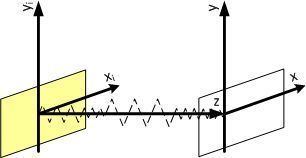
Electromagnetic wave propagation

Assuming the system looks like as depicted in the figure, the wave travels from plane x_i, y_i to the plane of x and y. The Fresnel transform is used to describe electromagnetic wave propagation in air:

U 0 ( x , y ) = − j λ e j k z z ∫ − ∞ ∞ ∫ − ∞ ∞ e j k 2 z [ ( x − x i ) 2 + ( y − y i ) 2 ] U i ( x i , y i ) d x i d y i ,

with

This is equivalent to LCT (shearing), when

[ a b c d ] = [ 1 λ z 0 1 ] .

When the travel distance (z) is larger, the shearing effect is larger.

Spherical lens

With the lens as depicted in the figure, and the refractive index denoted as n, the result is:

U 0 ( x , y ) = e j k n Δ e − j k 2 f [ x 2 + y 2 ] U i ( x , y )

with f the focal length and Δ the thickness of the lens.

The distortion passing through the lens is similar to LCT, when

[ a b c d ] = [ 1 0 − 1 λ f 1 ] .

This is also a shearing effect: when the focal length is smaller, the shearing effect is larger.

Spherical Mirror

The spherical mirror—e.g., a satellite dish—can be described as a LCT, with

[ a b c d ] = [ 1 0 − 1 λ R 1 ] .

This is very similar to lens, except focal length is replaced by the radius of the dish. Therefore, if the radius is smaller, the shearing effect is larger.

Example

The system considered is depicted in the figure to the right: two dishes – one being the emitter and the other one the receiver – and a signal travelling between them over a distance D. First, for dish A (emitter), the LCT matrix looks like this:

[ 1 0 − 1 λ R A 1 ] .

Then, for dish B (receiver), the LCT matrix similarly becomes:

[ 1 0 − 1 λ R B 1 ] .

Last, for the propagation of the signal in air, the LCT matrix is:

[ 1 λ D 0 1 ] .

Putting all three components together, the LCT of the system is:

[ a b c d ] = [ 1 0 − 1 λ R B 1 ] [ 1 λ D 0 1 ] [ 1 0 − 1 λ R A 1 ] = [ 1 − D R A − λ D 1 λ ( R A − 1 + R B − 1 − R A − 1 R B − 1 D ) 1 − D R B ] .

References

Linear canonical transformation Wikipedia

(Text) CC BY-SA

Contents