Radon transform - Alchetron, The Free Social Encyclopedia

In mathematics, the Radon transform is the integral transform which takes a function f defined on the plane to a function Rf defined on the (two-dimensional) space of lines in the plane, whose value at a particular line is equal to the line integral of the function over that line. The transform was introduced in 1917 by Johann Radon, who also provided a formula for the inverse transform. Radon further included formulas for the transform in three dimensions, in which the integral is taken over planes (integrating over lines is known as the X-ray transform). It was later generalized to higher-dimensional Euclidean spaces, and more broadly in the context of integral geometry. The complex analog of the Radon transform is known as the Penrose transform.The Radon transform is widely applicable to tomography, the creation of an image from the projection data associated with cross-sectional scans of an object.

Explanation

If a function f represents an unknown density, then the Radon transform represents the projection data obtained as the output of a tomographic scan. Hence the inverse of the Radon transform can be used to reconstruct the original density from the projection data, and thus it forms the mathematical underpinning for tomographic reconstruction, also known as image reconstruction.

The Radon transform data is often called a sinogram because the Radon transform of an off-center point source is a sinusoid. Consequently the Radon transform of a number of small objects appears graphically as a number of blurred sine waves with different amplitudes and phases.

The Radon transform is useful in computed axial tomography (CAT scan), barcode scanners, electron microscopy of macromolecular assemblies like viruses and protein complexes, reflection seismology and in the solution of hyperbolic partial differential equations.

Definition

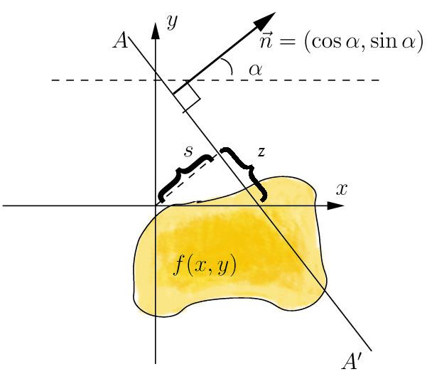
Let ƒ(x) = ƒ(x,y) be a compactly supported continuous function on R². The Radon transform, Rƒ, is a function defined on the space of straight lines L in R² by the line integral along each such line:

R f ( L ) = ∫ L f ( x ) | d x | .

Concretely, the parametrization of any straight line L with respect to arc length z can always be written

( x ( z ) , y ( z ) ) = ( ( z sin ⁡ α + s cos ⁡ α ) , ( − z cos ⁡ α + s sin ⁡ α ) )

where s is the distance of L from the origin and α is the angle the normal vector to L makes with the x axis. It follows that the quantities (α,s) can be considered as coordinates on the space of all lines in R², and the Radon transform can be expressed in these coordinates by

R f ( α , s ) = ∫ − ∞ ∞ f ( x ( z ) , y ( z ) ) d z = ∫ − ∞ ∞ f ( ( z sin ⁡ α + s cos ⁡ α ) , ( − z cos ⁡ α + s sin ⁡ α ) ) d z

More generally, in the n-dimensional Euclidean space Rⁿ, the Radon transform of a compactly supported continuous function ƒ is a function Rƒ on the space Σ_n of all hyperplanes in Rⁿ. It is defined by

R f ( ξ ) = ∫ ξ f ( x ) d σ ( x )

for ξ ∈Σ_n, where the integral is taken with respect to the natural hypersurface measure, dσ (generalizing the |dx| term from the 2-dimensional case). Observe that any element of Σ_n is characterized as the solution locus of an equation

x ⋅ α = s

where α ∈ Sⁿ⁻¹ is a unit vector and s ∈ R. Thus the n-dimensional Radon transform may be rewritten as a function on Sⁿ⁻¹×R via

R f ( α , s ) = ∫ x ⋅ α = s f ( x ) d σ ( x ) .

It is also possible to generalize the Radon transform still further by integrating instead over k-dimensional affine subspaces of Rⁿ. The X-ray transform is the most widely used special case of this construction, and is obtained by integrating over straight lines.

Relationship with the Fourier transform

The Radon transform is closely related to the Fourier transform. For a function of one variable the Fourier transform is defined by

f ^ ( ω ) = ∫ − ∞ ∞ f ( x ) e − 2 π i x ω d x .

and for a function of a 2-vector x = ( x , y ) ,

f ^ ( w ) = ∫ − ∞ ∞ ∫ − ∞ ∞ f ( x ) e − 2 π i x ⋅ w d x d y .

For convenience, denote R α [ f ] ( s ) = R [ f ] ( α , s ) . The Fourier slice theorem then states

R α [ f ] ^ ( σ ) = f ^ ( σ n ( α ) )

where

n ( α ) = ( cos ⁡ α , sin ⁡ α ) .

Thus the two-dimensional Fourier transform of the initial function along a line at the inclination angle α is the one variable Fourier transform of the Radon transform (acquired at angle α ) of that function.

More generally, one has the result valid in n dimensions

f ^ ( r α ) = ∫ − ∞ ∞ R f ( α , s ) e − 2 π i s r d s .

Dual transform

The dual Radon transform is a kind of adjoint to the Radon transform. Beginning with a function g on the space Σ_n, the dual Radon transform is the function R ∗ g on Rⁿ defined by

R ∗ g ( x ) = ∫ x ∈ ξ g ( ξ ) d μ ( ξ ) .

The integral here is taken over the set of all hyperplanes incident with the point x ∈ Rⁿ, and the measure dμ is the unique probability measure on the set { ξ | x ∈ ξ } invariant under rotations about the point x.

Concretely, for the two-dimensional Radon transform, the dual transform is given by

R ∗ g ( x ) = 1 2 π ∫ α = 0 2 π g ( α , n ( α ) ⋅ x ) d α .

In the context of image processing, the dual transform is commonly called backprojection as it takes a function defined on each line in the plane and 'smears' or projects it back over the line to produce an image.

Intertwining property

Let Δ denote the Laplacian on Rⁿ:

Δ = ∂ 2 ∂ x 1 2 + ⋯ + ∂ 2 ∂ x n 2 .

This is a natural rotationally invariant second-order differential operator. On Σ_n, the "radial" second derivative

L f ( α , s ) ≡ ∂ 2 ∂ s 2 f ( α , s )

is also rotationally invariant. The Radon transform and its dual are intertwining operators for these two differential operators in the sense that

R ( Δ f ) = L ( R f ) , R ∗ ( L g ) = Δ ( R ∗ g ) .

Reconstruction approaches

The process of reconstruction produces the image (or function f in the previous section) from its projection data. Reconstruction is an inverse problem.

Radon inversion formula

In the 2D case, the most commonly used analytical formula to recover f from its Radon transform is the Filtered Backprojection Formula or Radon Inversion Formula:

f ( x ) = ∫ 0 π ( R f ( ⋅ , θ ) ∗ h ) ( < x , n θ > ) d θ

where h is such that h ^ ( k ) = | k | .

The convolution kernel h is referred to as Ramp filter in some literature.

Ill-posedness

Intuitively, in the filtered backprojection formula, by analogy with differentiation, for which d d x ^ f ( k ) = i k f ^ ( k ) , we see that the filter performs an operation similar to a derivative. Roughly speaking, then, the filter makes objects more singular.

A quantitive statement of the ill-posedness of Radon Inversion goes as follows:

We have R ∗ R g ^ ( k ) = 1 | | k | | g ^ ( k )

where R ∗ is the previously defined adjoint to the Radon Transform.

Thus for g ( x ) = e i < k 0 , x > ,

R ∗ R g = 1 | | k 0 | | e i < k 0 , x > .

Iterative Reconstruction methods

Compared with the Filtered Backprojection method, iterative reconstruction costs large computation time, limiting its pratical use. However, due to the ill-posedness of Radon Inversion, the Filtered Backprojection method may be infeasible in the presence of discontinuity or noise. The iterative reconstruction could provide metal artifact reduction, noise and dose reduction for the reconstructed result that attract much research interest around the world.

Inversion formulas

Explicit and computationally efficient inversion formulas for the Radon transform and its dual are available. The Radon transform in n dimensions can be inverted by the formula

c n f = ( − Δ ) ( n − 1 ) / 2 R ∗ R f

where

c n = ( 4 π ) ( n − 1 ) / 2 Γ ( n / 2 ) Γ ( 1 / 2 ) .

and the power of the Laplacian (−Δ)^(n−1)/2 is defined as a pseudodifferential operator if necessary by the Fourier transform

F [ ( − Δ ) ( n − 1 ) / 2 ϕ ] ( ξ ) = | 2 π ξ | n − 1 F ϕ ( ξ ) .

For computational purposes, the power of the Laplacian is commuted with the dual transform R^* to give

c n f = { R ∗ d n − 1 d s n − 1 R f n o d d R ∗ H s d n − 1 d s n − 1 R f n e v e n

where H_s is the Hilbert transform with respect to the s variable. In two dimensions, the operator H_sd/ds appears in image processing as a ramp filter. One can prove directly from the Fourier slice theorem and change of variables for integration that for a compactly supported continuous function ƒ of two variables

f = 1 2 R ∗ H s d d s R f .

Thus in an image processing context the original image ƒ can be recovered from the 'sinogram' data Rƒ by applying a ramp filter (in the s variable) and then back-projecting. As the filtering step can be performed efficiently (for example using digital signal processing techniques) and the back projection step is simply an accumulation of values in the pixels of the image, this results in a highly efficient, and hence widely used, algorithm.

Explicitly, the inversion formula obtained by the latter method is

f ( x ) = 1 2 ( 2 π ) 1 − n ( − 1 ) ( n − 1 ) / 2 ∫ S n − 1 ∂ n − 1 ∂ s n − 1 R f ( α , α ⋅ x ) d α

if n is odd, and

f ( x ) = ( 2 π ) − n ( − 1 ) n / 2 ∫ − ∞ ∞ 1 q ∫ S n − 1 ∂ n − 1 ∂ s n − 1 R f ( α , α ⋅ x + q ) d α d q

if n is even.

The dual transform can also be inverted by an analogous formula:

c n g = ( − L ) ( n − 1 ) / 2 R ( R ∗ g ) .

References

Radon transform Wikipedia

(Text) CC BY-SA

Similar TopicsHeidi (2005 animated film)

Katherine L Adams

Elisabeth Rehn

Contents