Chirp - Alchetron, The Free Social Encyclopedia

A chirp is a signal in which the frequency increases (up-chirp) or decreases (down-chirp) with time. In some sources, the term chirp is used interchangeably with sweep signal. It is commonly used in sonar and radar, but has other applications, such as in spread-spectrum communications. In spread-spectrum usage, surface acoustic wave (SAW) devices such as reflective array compressors (RACs) are often used to generate and demodulate the chirped signals. In optics, ultrashort laser pulses also exhibit chirp, which, in optical transmission systems, interacts with the dispersion properties of the materials, increasing or decreasing total pulse dispersion as the signal propagates. The name is a reference to the chirping sound made by birds; see bird vocalization.

Definitions

If a waveform is defined as:

x ( t ) = sin ⁡ ( ϕ ( t ) )

then the instantaneous frequency is defined to be the phase rate:

f ( t ) = 1 2 π d ϕ ( t ) d t

and the (instantaneous) chirpyness is defined to be the frequency rate:

c ( t ) = 1 2 π d 2 ϕ ( t ) d t 2 = d f ( t ) d t

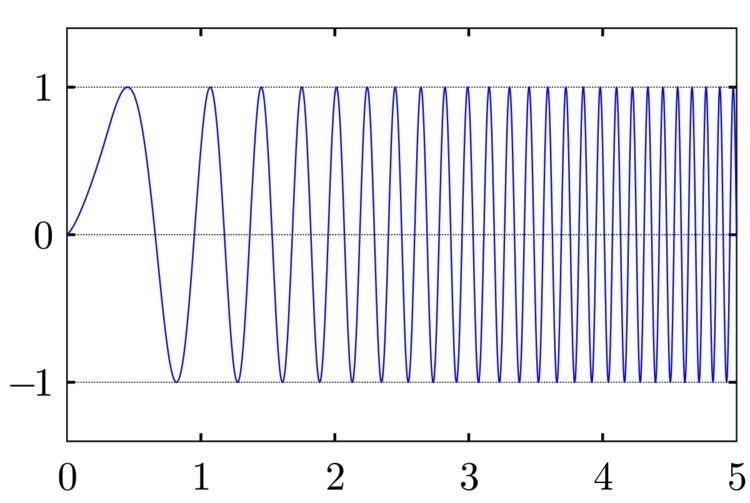
Linear

In a linear chirp, the instantaneous frequency f ( t ) varies exactly linearly with time:

f ( t ) = f 0 + k t ,

where f 0 is the starting frequency (at time t = 0 ), and k is the rate of frequency change or chirpyness.

k = f 1 − f 0 T ,

where f 1 is the final frequency and f 0 is the starting frequency. T is the time it takes to sweep from f 0 to f 1 .

The corresponding time-domain function for the phase of any oscillating signal is the integral of the frequency function, since one expects the phase to grow like ϕ ( t + Δ t ) ≃ ϕ ( t ) + 2 π f ( t ) Δ t , i.e., that the derivative of the phase is the angular frequency ϕ ′ ( t ) = 2 π f ( t ) .

For the linear chirp, this results in:

ϕ ( t ) = ϕ 0 + 2 π ∫ 0 t f ( τ ) d τ = ϕ 0 + 2 π ∫ 0 t ( f 0 + k τ ) d τ = ϕ 0 + 2 π ( f 0 t + k 2 t 2 ) ,

where ϕ 0 is the initial phase (at time t = 0 ). Thus this is also called quadratic-phase signal.

The corresponding time-domain function for a sinusoidal linear chirp is the sine of the phase in radians:

x ( t ) = sin ⁡ [ ϕ 0 + 2 π ( f 0 t + k 2 t 2 ) ]

Exponential

In a geometric chirp, also called an exponential chirp, the frequency of the signal varies with a geometric relationship over time. In other words, if two points in the waveform are chosen, t 1 and t 2 , and the time interval between them t 2 − t 1 is kept constant, the frequency ratio f ( t 2 ) / f ( t 1 ) will also be constant.

In an exponential chirp, the frequency of the signal varies exponentially as a function of time:

f ( t ) = f 0 k t

where f 0 is the starting frequency (at t = 0 ), and k is the rate of exponential change in frequency. Unlike the linear chirp, which has a constant chirpyness, an exponential chirp has an exponentially increasing frequency rate.

k = ( f 1 f 0 ) 1 T

The corresponding time-domain function for the phase of an exponential chirp is the integral of the frequency:

ϕ ( t ) = ϕ 0 + 2 π ∫ 0 t f ( τ ) d τ = ϕ 0 + 2 π f 0 ∫ 0 t k τ d τ = ϕ 0 + 2 π f 0 ( k t − 1 ln ⁡ ( k ) )

Where ϕ 0 is the initial phase (at t = 0 ).

The corresponding time-domain function for a sinusoidal exponential chirp is the sine of the phase in radians:

x ( t ) = sin ⁡ [ ϕ 0 + 2 π f 0 ( k t − 1 ln ⁡ ( k ) ) ]

As was the case for the Linear Chirp, the instantaneous frequency of the Exponential Chirp consists of the fundamental frequency f ( t ) = f 0 k t accompanied by additional harmonics.

Generation

A chirp signal can be generated with analog circuitry via a voltage-controlled oscillator (VCO), and a linearly or exponentially ramping control voltage. It can also be generated digitally by a digital signal processor (DSP) and digital to analog converter (DAC), using a direct digital synthesizer (DDS) and by varying the step in the numerically controlled oscillator. It can also be generated by a YIG oscillator.

Relation to an impulse signal

A chirp signal shares the same spectral content with an impulse signal. However, unlike in the impulse signal, spectral components of the chirp signal have different phases, i.e., their power spectra are alike but the phase spectra are distinct. Dispersion of a signal propagation medium may result in unintentional conversion of impulse signals into chirps. On the other hand, many practical applications, such as chirped pulse amplifiers or echolocation systems, use chirp signals instead of impulses because of their inherently lower PAPR.

Chirp modulation

Chirp modulation, or linear frequency modulation for digital communication, was patented by Sidney Darlington in 1954 with significant later work performed by Winkler in 1962. This type of modulation employs sinusoidal waveforms whose instantaneous frequency increases or decreases linearly over time. These waveforms are commonly referred to as linear chirps or simply chirps.

Hence the rate at which their frequency changes is called the chirp rate. In binary chirp modulation, binary data is transmitted by mapping the bits into chirps of opposite chirp rates. For instance, over one bit period "1" is assigned a chirp with positive rate a and "0" a chirp with negative rate −a. Chirps have been heavily used in radar applications and as a result advanced sources for transmission and matched filters for reception of linear chirps are available.

Chirplet transform

Another kind of chirp is the projective chirp, of the form:

g = f [ a ⋅ x + b c ⋅ x + 1 ] ,

having the three parameters a (scale), b (translation), and c (chirpiness). The projective chirp is ideally suited to image processing, and forms the basis for the projective chirplet transform.

Key chirp

A change in frequency of Morse code from the desired frequency, due to poor stability in the RF oscillator, is known as chirp, and in the RST code is given an appended letter 'C'.

References

Chirp Wikipedia

(Text) CC BY-SA

Contents