Trisha Shetty (Editor)

Empirical distribution function

Updated on
Edit
Like
Comment
Share on FacebookTweet on TwitterShare on LinkedInShare on Reddit
Empirical distribution function

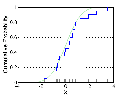
In statistics, an empirical distribution function is the distribution function associated with the empirical measure of a sample. This cumulative distribution function is a step function that jumps up by 1/n at each of the n data points. Its value at any specified value of the measured variable is the fraction of observations of the measured variable that are less than or equal to the specified value.

Contents

The empirical distribution function estimates the cumulative distribution function underlying of the points in the sample and converges with probability 1 according to the Glivenko–Cantelli theorem. A number of results exist to quantify the rate of convergence of the empirical distribution function to the underlying cumulative distribution function.

Definition

Let (x1, …, xn) be independent, identically distributed real random variables with the common cumulative distribution function F(t). Then the empirical distribution function is defined as

F ^ n ( t ) = number of elements in the sample t n = 1 n i = 1 n 1 x i t ,

where 1 A is the indicator of event A. For a fixed t, the indicator 1 x i t is a Bernoulli random variable with parameter p = F(t), hence n F ^ n ( t ) is a binomial random variable with mean nF(t) and variance nF(t)(1 − F(t)). This implies that F ^ n ( t ) is an unbiased estimator for F(t).

However, in some textbooks, the definition is given as F ^ n ( t ) = 1 n + 1 i = 1 n 1 x i t

Asymptotic properties

Since the ratio (n+1) / n approaches 1 as n goes to infinity, the asymptotic properties of the two definitions that are given above are the same.

By the strong law of large numbers, the estimator F ^ n ( t ) converges to F(t) as almost surely, for every value of t:

F ^ n ( t )   a . s .   F ( t ) ,

thus the estimator F ^ n ( t ) is consistent. This expression asserts the pointwise convergence of the empirical distribution function to the true cumulative distribution function. There is a stronger result, called the Glivenko–Cantelli theorem, which states that the convergence in fact happens uniformly over t:

F ^ n F sup t R | F ^ n ( t ) F ( t ) |   a . s .   0.

The sup-norm in this expression is called the Kolmogorov–Smirnov statistic for testing the goodness-of-fit between the empirical distribution F ^ n ( t ) and the assumed true cumulative distribution function F. Other norm functions may be reasonably used here instead of the sup-norm. For example, the L²-norm gives rise to the Cramér–von Mises statistic.

The asymptotic distribution can be further characterized in several different ways. First, the central limit theorem states that pointwise, F ^ n ( t ) has asymptotically normal distribution with the standard n rate of convergence:

n ( F ^ n ( t ) F ( t ) )     d     N ( 0 , F ( t ) ( 1 F ( t ) ) ) .

This result is extended by the Donsker’s theorem, which asserts that the empirical process n ( F ^ n F ) , viewed as a function indexed by t R , converges in distribution in the Skorokhod space D [ , + ] to the mean-zero Gaussian process G F = B F , where B is the standard Brownian bridge. The covariance structure of this Gaussian process is

E [ G F ( t 1 ) G F ( t 2 ) ] = F ( t 1 t 2 ) F ( t 1 ) F ( t 2 ) .

The uniform rate of convergence in Donsker’s theorem can be quantified by the result known as the Hungarian embedding:

lim sup n n ln 2 n n ( F ^ n F ) G F , n < , a.s.

Alternatively, the rate of convergence of n ( F ^ n F ) can also be quantified in terms of the asymptotic behavior of the sup-norm of this expression. Number of results exist in this venue, for example the Dvoretzky–Kiefer–Wolfowitz inequality provides bound on the tail probabilities of n F ^ n F :

Pr ( n F ^ n F > z ) 2 e 2 z 2 .

In fact, Kolmogorov has shown that if the cumulative distribution function F is continuous, then the expression n F ^ n F converges in distribution to B , which has the Kolmogorov distribution that does not depend on the form of F.

Another result, which follows from the law of the iterated logarithm, is that

lim sup n n F ^ n F 2 ln ln n 1 2 , a.s.

and

lim inf n 2 n ln ln n F ^ n F = π 2 , a.s.

References

Empirical distribution function Wikipedia