Law of the iterated logarithm

Statement

Let {Y_n} be independent, identically distributed random variables with means zero and unit variances. Let S_n = Y₁ + … + Y_n. Then

where “log” is the natural logarithm, “lim sup” denotes the limit superior, and “a.s.” stands for “almost surely”.

Discussion

The law of iterated logarithms operates “in between” the law of large numbers and the central limit theorem. There are two versions of the law of large numbers — the weak and the strong — and they both state that the sums S_n, scaled by n⁻¹, converge to zero, respectively in probability and almost surely:

On the other hand, the central limit theorem states that the sums S_n scaled by the factor n^−½ converge in distribution to a standard normal distribution. By Kolmogorov's zero-one law, for any fixed M, the probability that the event lim sup n S n n > M occurs is 0 or 1. Then

so

An identical argument shows that

This implies that these quantities cannot converge almost surely. In fact, they cannot even converge in probability, which follows from the equality

and the fact that the random variables

are independent and both converge in distribution to N ( 0 , 1 ) .

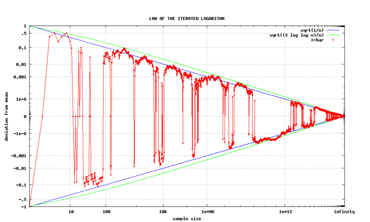
The law of the iterated logarithm provides the scaling factor where the two limits become different:

Thus, although the quantity S n / n log ⁡ log ⁡ n is less than any predefined ε > 0 with probability approaching one, that quantity will nevertheless be dropping out of that interval infinitely often, and in fact will be visiting the neighborhoods of any point in the interval (-√2,√2) almost surely.

Generalizations and variants

The law of the iterated logarithm (LIL) for a sum of independent and identically distributed (i.i.d.) random variables with zero mean and bounded increment dates back to Khinchin and Kolmogorov in the 1920s.

Since then, there has been a tremendous amount of work on the LIL for various kinds of dependent structures and for stochastic processes. Following is a small sample of notable developments.

Hartman-Wintner (1940) generalized LIL to random walks with increments with zero mean and finite variance.

Strassen (1964) studied LIL from the point of view of invariance principles.

Stout (1970) generalized the LIL to stationary ergodic martingales.

de Acosta (1983) gave a simple proof of Hartman-Wintner version of LIL.

Wittmann (1985) generalized Hartman-Wintner version of LIL to random walks satisfying milder conditions.

Vovk (1987) derived a version of LIL valid for a single chaotic sequence (Kolmogorov random sequence). This is notable as it is outside the realm of classical probability theory.

The law of iterated logarithm for pseudo-randomness

Yongge Wang has shown that the law of the iterated logarithm holds for polynomial time pseudorandom sequences also. Furthermore, the Java based software testing tool statistical testing techniques for pseudorandom generation is available for testing whether a randomness generator outputs sequences that satisfy the LIL.