Gaussian process

Definition

A Gaussian process is a statistical distribution X_t, t ∈ T, for which any finite linear combination of samples has a joint Gaussian distribution. More accurately, any linear functional applied to the sample function X_t will give a normally distributed result. Notation-wise, one can write X ~ GP(m,K), meaning the random function X is distributed as a GP with mean function m and covariance function K. When the input vector t is two- or multi-dimensional, a Gaussian process might be also known as a Gaussian random field.

Some authors assume the random variables X_t have mean zero; this simplifies calculations without loss of generality and allows the mean square properties of the process to be entirely determined by the covariance function K.

Alternative definitions

Alternatively, a time continuous stochastic process is Gaussian if and only if for every finite set of indices t 1 , … , t k in the index set T

is a multivariate Gaussian random variable. Using characteristic functions of random variables, the Gaussian property can be formulated as follows: { X t ; t ∈ T } is Gaussian if and only if, for every finite set of indices t 1 , … , t k , there are real valued σ ℓ j , μ ℓ with σ j j > 0 such that the following equality holds for all s 1 , s 2 , . . . s k ∈ R

where i denotes the imaginary number − 1 .

The numbers σ ℓ j and μ ℓ can be shown to be the covariances and means of the variables in the process.

Covariance functions

A key fact of Gaussian processes is that they can be completely defined by their second-order statistics. Thus, if a Gaussian process is assumed to have mean zero, defining the covariance function completely defines the process' behaviour. Importantly the non-negative definiteness of this function enables its spectral decomposition using the Karhunen–Loeve expansion. Basic aspects that can be defined through the covariance function are the process' stationarity, isotropy, smoothness and periodicity.

Stationarity refers to the process' behaviour regarding the separation of any two points x and x' . If the process is stationary, it depends on their separation, x − x', while if non-stationary it depends on the actual position of the points x and x'. For example, the special case of an Ornstein–Uhlenbeck process, a Brownian motion process, is stationary.

If the process depends only on |x − x'|, the Euclidean distance (not the direction) between x and x', then the process is considered isotropic. A process that is concurrently stationary and isotropic is considered to be homogeneous; in practice these properties reflect the differences (or rather the lack of them) in the behaviour of the process given the location of the observer.

Ultimately Gaussian processes translate as taking priors on functions and the smoothness of these priors can be induced by the covariance function. If we expect that for "near-by" input points x and x' their corresponding output points y and y' to be "near-by" also, then the assumption of continuity is present. If we wish to allow for significant displacement then we might choose a rougher covariance function. Extreme examples of the behaviour is the Ornstein–Uhlenbeck covariance function and the squared exponential where the former is never differentiable and the latter infinitely differentiable.

Periodicity refers to inducing periodic patterns within the behaviour of the process. Formally, this is achieved by mapping the input x to a two dimensional vector u(x) = (cos(x), sin(x)).

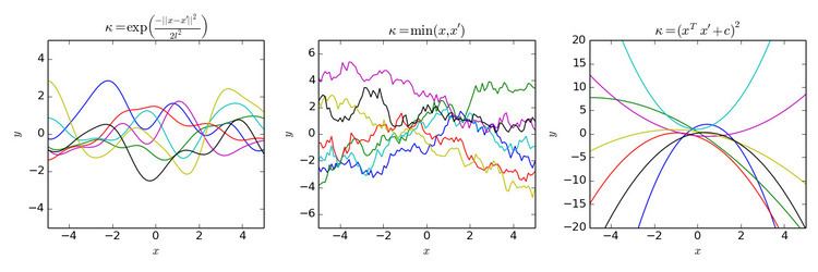
Usual covariance functions

There are a number of common covariance functions:

Here d = x − x ′ . The parameter l is the characteristic length-scale of the process (practically, "how close" two points x and x ′ have to be to influence each other significantly), δ is the Kronecker delta and σ the standard deviation of the noise fluctuations. Moreover, K ν is the modified Bessel function of order ν and Γ ( ν ) is the gamma function evaluated at ν . Importantly, a complicated covariance function can be defined as a linear combination of other simpler covariance functions in order to incorporate different insights about the data-set at hand.

Clearly, the inferential results are dependent on the values of the hyperparameters θ (e.g. l and σ) defining the model's behaviour. A popular choice for θ is to provide maximum a posteriori (MAP) estimates of it with some chosen prior. If the prior is very near uniform, this is the same as maximizing the marginal likelihood of the process; the marginalization being done over the observed process values y . This approach is also known as maximum likelihood II, evidence maximization, or Empirical Bayes.

Brownian Motion as the Integral of Gaussian processes

A Wiener process (aka Brownian motion) is the integral of a white noise Gaussian process. It is not stationary, but it has stationary increments.

The Ornstein–Uhlenbeck process is a stationary Gaussian process.

The Brownian bridge is the integral of a Gaussian process whose increments are not independent.

The fractional Brownian motion is the integral of a Gaussian process whose covariance function is a generalisation of Wiener process.

Applications

A Gaussian process can be used as a prior probability distribution over functions in Bayesian inference. Given any set of N points in the desired domain of your functions, take a multivariate Gaussian whose covariance matrix parameter is the Gram matrix of your N points with some desired kernel, and sample from that Gaussian.

Inference of continuous values with a Gaussian process prior is known as Gaussian process regression, or kriging; extending Gaussian process regression to multiple target variables is known as cokriging. Gaussian processes are thus useful as a powerful non-linear multivariate interpolation tool. Gaussian process regression can be further extended to address learning tasks in both supervised (e.g. probabilistic classification) and unsupervised (e.g. manifold learning) learning frameworks.

Gaussian process prediction, or kriging

When concerned with a general Gaussian process regression problem (kriging), it is assumed that for a Gaussian process f observed at coordinates x, the vector of values f ( x ) is just one sample from a multivariate Gaussian distribution of dimension equal to number of observed coordinates |x|. Therefore, under the assumption of a zero-mean distribution, f ( x ) ∼ N ( 0 , K ( θ , x , x ′ ) ) , where K ( θ , x , x ′ ) is the covariance matrix between all possible pairs ( x , x ′ ) for a given set of hyperparameters θ. As such the log marginal likelihood is:

and maximizing this marginal likelihood towards θ provides the complete specification of the Gaussian process f. One can briefly note at this point that the first term corresponds to a penalty term for a model's failure to fit observed values and the second term to a penalty term that increases proportionally to a model's complexity. Having specified θ making predictions about unobserved values f ( x ∗ ) at coordinates x* is then only a matter of drawing samples from the predictive distribution p ( y ∗ | x ∗ , f ( x ) , x ) = N ( y ∗ | A , B ) where the posterior mean estimate A is defined as:

and the posterior variance estimate B is defined as:

where K ( θ , x ∗ , x ′ ) is the covariance between the new coordinate of estimation x* and all other observed coordinates x for a given hyperparameter vector θ, K ( θ , x , x ′ ) and f ( x ) are defined as before and K ( θ , x ∗ , x ∗ ) is the variance at point x* as dictated by θ. It is important to note that practically the posterior mean estimate f ( x ∗ ) (the "point estimate") is just a linear combination of the observations f ( x ) ; in a similar manner the variance of f ( x ∗ ) is actually independent of the observations f ( x ) . A known bottleneck in Gaussian process prediction is that the computational complexity of prediction is cubic in the number of points |x| and as such can become unfeasible for larger data sets. Works on sparse Gaussian processes, that usually are based on the idea of building a representative set for the given process f, try to circumvent this issue.