Kolmogorov–Smirnov test - Alchetron, the free social encyclopedia

In statistics, the Kolmogorov–Smirnov test (K–S test or KS test) is a nonparametric test of the equality of continuous, one-dimensional probability distributions that can be used to compare a sample with a reference probability distribution (one-sample K–S test), or to compare two samples (two-sample K–S test). The Kolmogorov–Smirnov statistic quantifies a distance between the empirical distribution function of the sample and the cumulative distribution function of the reference distribution, or between the empirical distribution functions of two samples. The null distribution of this statistic is calculated under the null hypothesis that the sample is drawn from the reference distribution (in the one-sample case) or that the samples are drawn from the same distribution (in the two-sample case). In each case, the distributions considered under the null hypothesis are continuous distributions but are otherwise unrestricted.

The Kolmogorov–Smirnov test can be modified to serve as a goodness of fit test. In the special case of testing for normality of the distribution, samples are standardized and compared with a standard normal distribution. This is equivalent to setting the mean and variance of the reference distribution equal to the sample estimates, and it is known that using these to define the specific reference distribution changes the null distribution of the test statistic: see below. Various studies have found that, even in this corrected form, the test is less powerful for testing normality than the Shapiro–Wilk test or Anderson–Darling test. However, these other tests have their own disadvantages. For instance the Shapiro–Wilk test is known to not work well with many ties (many identical values).

Kolmogorov–Smirnov statistic

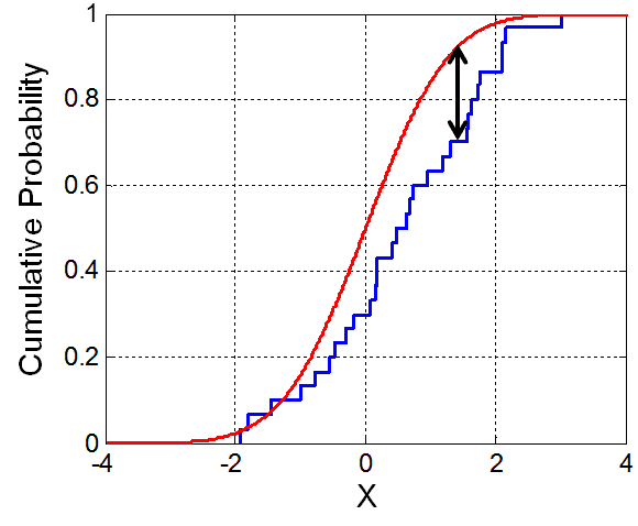
The empirical distribution function F_n for n iid observations X_i is defined as

F n ( x ) = 1 n ∑ i = 1 n I [ − ∞ , x ] ( X i )

where I [ − ∞ , x ] ( X i ) is the indicator function, equal to 1 if X i ≤ x and equal to 0 otherwise.

The Kolmogorov–Smirnov statistic for a given cumulative distribution function F(x) is

D n = sup x | F n ( x ) − F ( x ) |

where sup _x is the supremum of the set of distances. By the Glivenko–Cantelli theorem, if the sample comes from distribution F(x), then D_n converges to 0 almost surely in the limit when n goes to infinity. Kolmogorov strengthened this result, by effectively providing the rate of this convergence (see below). Donsker's theorem provides yet a stronger result.

In practice, the statistic requires a relatively large number of data points to properly reject the null hypothesis.

Kolmogorov distribution

The Kolmogorov distribution is the distribution of the random variable

K = sup t ∈ [ 0 , 1 ] | B ( t ) |

where B(t) is the Brownian bridge. The cumulative distribution function of K is given by

Pr ⁡ ( K ≤ x ) = 1 − 2 ∑ k = 1 ∞ ( − 1 ) k − 1 e − 2 k 2 x 2 = 2 π x ∑ k = 1 ∞ e − ( 2 k − 1 ) 2 π 2 / ( 8 x 2 ) ,

which can also be expressed by the Jacobi theta function ϑ 01 ( z = 0 ; τ = 2 i x 2 / π ) . Both the form of the Kolmogorov–Smirnov test statistic and its asymptotic distribution under the null hypothesis were published by Andrey Kolmogorov, while a table of the distribution was published by Nikolai Vasilyevich Smirnov. Recurrence relations for the distribution of the test statistic in finite samples are available.

Under null hypothesis that the sample comes from the hypothesized distribution F(x),

n D n → n → ∞ sup t | B ( F ( t ) ) |

in distribution, where B(t) is the Brownian bridge.

If F is continuous then under the null hypothesis n D n converges to the Kolmogorov distribution, which does not depend on F. This result may also be known as the Kolmogorov theorem; see Kolmogorov's theorem for disambiguation.

The goodness-of-fit test or the Kolmogorov–Smirnov test is constructed by using the critical values of the Kolmogorov distribution. The null hypothesis is rejected at level α if

n D n > K α ,

where K_α is found from

Pr ⁡ ( K ≤ K α ) = 1 − α .

The asymptotic power of this test is 1.

Test with estimated parameters

If either the form or the parameters of F(x) are determined from the data X_i the critical values determined in this way are invalid. In such cases, Monte Carlo or other methods may be required, but tables have been prepared for some cases. Details for the required modifications to the test statistic and for the critical values for the normal distribution and the exponential distribution have been published, and later publications also include the Gumbel distribution. The Lilliefors test represents a special case of this for the normal distribution. The logarithm transformation may help to overcome cases where the Kolmogorov test data does not seem to fit the assumption that it came from the normal distribution.

Discrete null distribution

The Kolmogorov–Smirnov test must be adapted for discrete variables. The form of the test statistic remains the same as in the continuous case, but the calculation of its value is more subtle. We can see this if we consider computing the test statistic between a continuous distribution f ( x ) and a step function g ( x ) that has a discontinuity at x i . In other words, the limit lim x → x i g ( x ) , if it exists, is different from g ( x i ) . Thus, when computing the statistic

it is unclear how to replace the limit, unless we know the limiting value of the underlying distribution.

In SAS, the Kolmogorov–Smirnov test is implemented in PROC NPAR1WAY. The discretized KS test is implemented in the ks.test() function in the dgof package of the R project for statistical computing. In Stata, the command ksmirnov performs a Kolmogorov–Smirnov test.

Two-sample Kolmogorov–Smirnov test

The Kolmogorov–Smirnov test may also be used to test whether two underlying one-dimensional probability distributions differ. In this case, the Kolmogorov–Smirnov statistic is

D n , n ′ = sup x | F 1 , n ( x ) − F 2 , n ′ ( x ) | ,

where F 1 , n and F 2 , n ′ are the empirical distribution functions of the first and the second sample respectively, and sup is the supremum function.

The null hypothesis is rejected at level α if

D n , n ′ > c ( α ) n + n ′ n n ′ .

Where n and n ′ are the sizes of first and second sample respectively. The value of c ( α ) is given in the table below for the most common levels of α

and in general by

c ( α ) = − 1 2 ln ⁡ ( α 2 ) .

Note that the two-sample test checks whether the two data samples come from the same distribution. This does not specify what that common distribution is (e.g. whether it's normal or not normal). Again, tables of critical values have been published. These critical values have one thing in common with the Anderson–Darling and Chi-squares, namely the fact that higher values tend to be more rare.

Setting confidence limits for the shape of a distribution function

While the Kolmogorov–Smirnov test is usually used to test whether a given F(x) is the underlying probability distribution of F_n(x), the procedure may be inverted to give confidence limits on F(x) itself. If one chooses a critical value of the test statistic D_α such that P(D_n > D_α) = α, then a band of width ±D_α around F_n(x) will entirely contain F(x) with probability 1 − α.

The Kolmogorov–Smirnov statistic in more than one dimension

A distribution-free multivariate Kolmogorov–Smirnov goodness of fit test has been proposed by Justel, Peña and Zamar (1997). The test uses a statistic which is built using Rosenblatt's transformation, and an algorithm is developed to compute it in the bivariate case. An approximate test that can be easily computed in any dimension is also presented.

The Kolmogorov–Smirnov test statistic needs to be modified if a similar test is to be applied to multivariate data. This is not straightforward because the maximum difference between two joint cumulative distribution functions is not generally the same as the maximum difference of any of the complementary distribution functions. Thus the maximum difference will differ depending on which of Pr ( x < X ∧ y < Y ) or Pr ( X < x ∧ Y > y ) or any of the other two possible arrangements is used. One might require that the result of the test used should not depend on which choice is made.

One approach to generalizing the Kolmogorov–Smirnov statistic to higher dimensions which meets the above concern is to compare the cdfs of the two samples with all possible orderings, and take the largest of the set of resulting K–S statistics. In d dimensions, there are 2^d−1 such orderings. One such variation is due to Peacock and another to Fasano and Franceschini (see Lopes et al. for a comparison and computational details). Critical values for the test statistic can be obtained by simulations, but depend on the dependence structure in the joint distribution.

References

Kolmogorov–Smirnov test Wikipedia

(Text) CC BY-SA

Contents