Chaos theory

Introduction

Chaos theory concerns deterministic systems whose behavior can in principle be predicted. Chaotic systems are predictable for a while and then 'appear' to become random. The amount of time that the behavior of a chaotic system can be effectively predicted depends on three things: How much uncertainty we tolerate in the forecast, how accurately we can measure its current state, and a time scale depending on the dynamics of the system, called the Lyapunov time. Some examples of Lyapunov times are: chaotic electrical circuits, about 1 millisecond; weather systems, a few days (unproven); the solar system, 50 million years. In chaotic systems, the uncertainty in a forecast increases exponentially with elapsed time. Hence, mathematically, doubling the forecast time more than squares the proportional uncertainty in the forecast. This means, in practice, a meaningful prediction cannot be made over an interval of more than two or three times the Lyapunov time. When meaningful predictions cannot be made, the system appears random.

Chaotic dynamics

In common usage, "chaos" means "a state of disorder". However, in chaos theory, the term is defined more precisely. Although no universally accepted mathematical definition of chaos exists, a commonly used definition originally formulated by Robert L. Devaney says that, to classify a dynamical system as chaotic, it must have these properties:

1. it must be sensitive to initial conditions
2. it must be topologically mixing
3. it must have dense periodic orbits

In some cases, the last two properties in the above have been shown to actually imply sensitivity to initial conditions. In these cases, while it is often the most practically significant property, "sensitivity to initial conditions" need not be stated in the definition.

If attention is restricted to intervals, the second property implies the other two. An alternative, and in general weaker, definition of chaos uses only the first two properties in the above list.

Sensitivity to initial conditions

Sensitivity to initial conditions means that each point in a chaotic system is arbitrarily closely approximated by other points with significantly different future paths, or trajectories. Thus, an arbitrarily small change, or perturbation, of the current trajectory may lead to significantly different future behavior.

Sensitivity to initial conditions is popularly known as the "butterfly effect", so-called because of the title of a paper given by Edward Lorenz in 1972 to the American Association for the Advancement of Science in Washington, D.C., entitled Predictability: Does the Flap of a Butterfly's Wings in Brazil set off a Tornado in Texas?. The flapping wing represents a small change in the initial condition of the system, which causes a chain of events leading to large-scale phenomena. Had the butterfly not flapped its wings, the trajectory of the system might have been vastly different.

A consequence of sensitivity to initial conditions is that if we start with only a finite amount of information about the system (as is usually the case in practice), then beyond a certain time the system is no longer predictable. This is most familiar in the case of weather, which is generally predictable only about a week ahead. Of course, this does not mean that we cannot say anything about events far in the future; some restrictions on the system are present. With weather, we know that the temperature will never naturally reach 100 °C or fall to -130 °C on earth, but we can't say exactly what day will have the hottest temperature of the year.

In more mathematical terms, the Lyapunov exponent measures the sensitivity to initial conditions. Given two starting trajectories in the phase space that are infinitesimally close, with initial separation δ Z 0 , the two trajectories end up diverging at a rate given by

where t is the time and λ is the Lyapunov exponent. The rate of separation depends on the orientation of the initial separation vector, so a whole spectrum of Lyapunov exponents exist. The number of Lyapunov exponents is equal to the number of dimensions of the phase space, though it is common to just refer to the largest one. For example, the maximal Lyapunov exponent (MLE) is most often used because it determines the overall predictability of the system. A positive MLE is usually taken as an indication that the system is chaotic.

Also, other properties relate to sensitivity of initial conditions, such as measure-theoretical mixing (as discussed in ergodic theory) and properties of a K-system.

Topological mixing

Topological mixing (or topological transitivity) means that the system evolves over time so that any given region or open set of its phase space eventually overlaps with any other given region. This mathematical concept of "mixing" corresponds to the standard intuition, and the mixing of colored dyes or fluids is an example of a chaotic system.

Topological mixing is often omitted from popular accounts of chaos, which equate chaos with only sensitivity to initial conditions. However, sensitive dependence on initial conditions alone does not give chaos. For example, consider the simple dynamical system produced by repeatedly doubling an initial value. This system has sensitive dependence on initial conditions everywhere, since any pair of nearby points eventually becomes widely separated. However, this example has no topological mixing, and therefore has no chaos. Indeed, it has extremely simple behavior: all points except 0 tend to positive or negative infinity.

Density of periodic orbits

For a chaotic system to have dense periodic orbits means that every point in the space is approached arbitrarily closely by periodic orbits. The one-dimensional logistic map defined by x → 4 x (1 – x) is one of the simplest systems with density of periodic orbits. For example, 5 − 5 8  → 5 + 5 8  → 5 − 5 8 (or approximately 0.3454915 → 0.9045085 → 0.3454915) is an (unstable) orbit of period 2, and similar orbits exist for periods 4, 8, 16, etc. (indeed, for all the periods specified by Sharkovskii's theorem).

Sharkovskii's theorem is the basis of the Li and Yorke (1975) proof that any one-dimensional system that exhibits a regular cycle of period three will also display regular cycles of every other length, as well as completely chaotic orbits.

Strange attractors

Some dynamical systems, like the one-dimensional logistic map defined by x → 4 x (1 – x), are chaotic everywhere, but in many cases chaotic behavior is found only in a subset of phase space. The cases of most interest arise when the chaotic behavior takes place on an attractor, since then a large set of initial conditions leads to orbits that converge to this chaotic region.

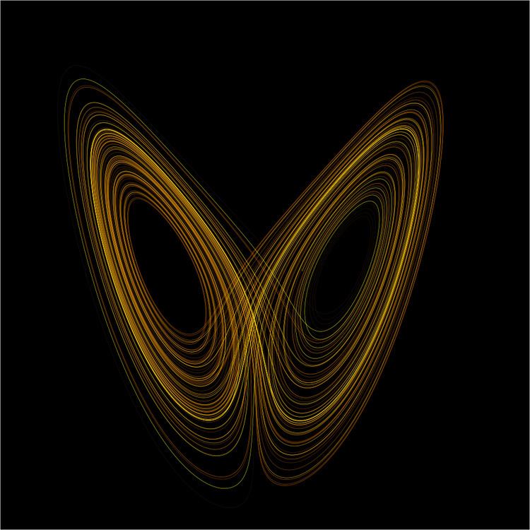
An easy way to visualize a chaotic attractor is to start with a point in the basin of attraction of the attractor, and then simply plot its subsequent orbit. Because of the topological transitivity condition, this is likely to produce a picture of the entire final attractor, and indeed both orbits shown in the figure on the right give a picture of the general shape of the Lorenz attractor. This attractor results from a simple three-dimensional model of the Lorenz weather system. The Lorenz attractor is perhaps one of the best-known chaotic system diagrams, probably because it was not only one of the first, but it is also one of the most complex and as such gives rise to a very interesting pattern, that with a little imagination, looks like the wings of a butterfly.

Unlike fixed-point attractors and limit cycles, the attractors that arise from chaotic systems, known as strange attractors, have great detail and complexity. Strange attractors occur in both continuous dynamical systems (such as the Lorenz system) and in some discrete systems (such as the Hénon map). Other discrete dynamical systems have a repelling structure called a Julia set, which forms at the boundary between basins of attraction of fixed points. Julia sets can be thought of as strange repellers. Both strange attractors and Julia sets typically have a fractal structure, and the fractal dimension can be calculated for them.

Minimum complexity of a chaotic system

Discrete chaotic systems, such as the logistic map, can exhibit strange attractors whatever their dimensionality. In contrast, for continuous dynamical systems, the Poincaré–Bendixson theorem shows that a strange attractor can only arise in three or more dimensions. Finite-dimensional linear systems are never chaotic; for a dynamical system to display chaotic behavior, it must be either nonlinear or infinite-dimensional.

The Poincaré–Bendixson theorem states that a two-dimensional differential equation has very regular behavior. The Lorenz attractor discussed above is generated by a system of three differential equations such as:

where x , y , and z make up the system state, t is time, and σ , ρ , β are the system parameters. Five of the terms on the right hand side are linear, while two are quadratic; a total of seven terms. Another well-known chaotic attractor is generated by the Rössler equations, which have only one nonlinear term out of seven. Sprott found a three-dimensional system with just five terms, that had only one nonlinear term, which exhibits chaos for certain parameter values. Zhang and Heidel showed that, at least for dissipative and conservative quadratic systems, three-dimensional quadratic systems with only three or four terms on the right-hand side cannot exhibit chaotic behavior. The reason is, simply put, that solutions to such systems are asymptotic to a two-dimensional surface and therefore solutions are well behaved.

While the Poincaré–Bendixson theorem shows that a continuous dynamical system on the Euclidean plane cannot be chaotic, two-dimensional continuous systems with non-Euclidean geometry can exhibit chaotic behavior. Perhaps surprisingly, chaos may occur also in linear systems, provided they are infinite dimensional. A theory of linear chaos is being developed in a branch of mathematical analysis known as functional analysis.

Jerk systems

In physics, jerk is the third derivative of position, with respect to time. As such, differential equations of the form

are sometimes called Jerk equations. It has been shown, that a jerk equation, which is equivalent to a system of three first order, ordinary, non-linear differential equations is in a certain sense the minimal setting for solutions showing chaotic behaviour. This motivates mathematical interest in jerk systems. Systems involving a fourth or higher derivative are called accordingly hyperjerk systems.

A jerk system's behavior is described by a jerk equation, and for certain jerk equations, simple electronic circuits can model solutions. These circuits are known as jerk circuits.

One of the most interesting properties of jerk circuits is the possibility of chaotic behavior. In fact, certain well-known chaotic systems, such as the Lorenz attractor and the Rössler map, are conventionally described as a system of three first-order differential equations that can combine into a single (although rather complicated) jerk equation. Nonlinear jerk systems are in a sense minimally complex systems to show chaotic behaviour, there is no chaotic system involving only two first-order, ordinary differential equations (the system resulting in an equation of second order only).

An example of a jerk equation with nonlinearity in the magnitude of x is:

Here, A is an adjustable parameter. This equation has a chaotic solution for A=3/5 and can be implemented with the following jerk circuit; the required nonlinearity is brought about by the two diodes:

In the above circuit, all resistors are of equal value, except R A = R / A = 5 R / 3 , and all capacitors are of equal size. The dominant frequency is 1 / 2 π R C . The output of op amp 0 will correspond to the x variable, the output of 1 corresponds to the first derivative of x and the output of 2 corresponds to the second derivative.

Spontaneous order

Under the right conditions, chaos spontaneously evolves into a lockstep pattern. In the Kuramoto model, four conditions suffice to produce synchronization in a chaotic system. Examples include the coupled oscillation of Christiaan Huygens' pendulums, fireflies, neurons, the London Millennium Bridge resonance, and large arrays of Josephson junctions.

History

An early proponent of chaos theory was Henri Poincaré. In the 1880s, while studying the three-body problem, he found that there can be orbits that are nonperiodic, and yet not forever increasing nor approaching a fixed point. In 1898 Jacques Hadamard published an influential study of the chaotic motion of a free particle gliding frictionlessly on a surface of constant negative curvature, called "Hadamard's billiards". Hadamard was able to show that all trajectories are unstable, in that all particle trajectories diverge exponentially from one another, with a positive Lyapunov exponent.

Chaos theory got its start in the field of ergodic theory. Later studies, also on the topic of nonlinear differential equations, were carried out by George David Birkhoff, Andrey Nikolaevich Kolmogorov, Mary Lucy Cartwright and John Edensor Littlewood, and Stephen Smale. Except for Smale, these studies were all directly inspired by physics: the three-body problem in the case of Birkhoff, turbulence and astronomical problems in the case of Kolmogorov, and radio engineering in the case of Cartwright and Littlewood. Although chaotic planetary motion had not been observed, experimentalists had encountered turbulence in fluid motion and nonperiodic oscillation in radio circuits without the benefit of a theory to explain what they were seeing.

Despite initial insights in the first half of the twentieth century, chaos theory became formalized as such only after mid-century, when it first became evident to some scientists that linear theory, the prevailing system theory at that time, simply could not explain the observed behavior of certain experiments like that of the logistic map. What had been attributed to measure imprecision and simple "noise" was considered by chaos theorists as a full component of the studied systems.

The main catalyst for the development of chaos theory was the electronic computer. Much of the mathematics of chaos theory involves the repeated iteration of simple mathematical formulas, which would be impractical to do by hand. Electronic computers made these repeated calculations practical, while figures and images made it possible to visualize these systems. As a graduate student in Chihiro Hayashi's laboratory at Kyoto University, Yoshisuke Ueda was experimenting with analog computers and noticed, on Nov. 27, 1961, what he called "randomly transitional phenomena". Yet his advisor did not agree with his conclusions at the time, and did not allow him to report his findings until 1970.

Edward Lorenz was an early pioneer of the theory. His interest in chaos came about accidentally through his work on weather prediction in 1961. Lorenz was using a simple digital computer, a Royal McBee LGP-30, to run his weather simulation. He wanted to see a sequence of data again, and to save time he started the simulation in the middle of its course. He did this by entering a printout of the data that corresponded to conditions in the middle of the original simulation. To his surprise, the weather the machine began to predict was completely different from the previous calculation. Lorenz tracked this down to the computer printout. The computer worked with 6-digit precision, but the printout rounded variables off to a 3-digit number, so a value like 0.506127 printed as 0.506. This difference is tiny, and the consensus at the time would have been that it should have no practical effect. However, Lorenz discovered that small changes in initial conditions produced large changes in long-term outcome. Lorenz's discovery, which gave its name to Lorenz attractors, showed that even detailed atmospheric modelling cannot, in general, make precise long-term weather predictions.

In 1963, Benoit Mandelbrot found recurring patterns at every scale in data on cotton prices. Beforehand he had studied information theory and concluded noise was patterned like a Cantor set: on any scale the proportion of noise-containing periods to error-free periods was a constant – thus errors were inevitable and must be planned for by incorporating redundancy. Mandelbrot described both the "Noah effect" (in which sudden discontinuous changes can occur) and the "Joseph effect" (in which persistence of a value can occur for a while, yet suddenly change afterwards). This challenged the idea that changes in price were normally distributed. In 1967, he published "How long is the coast of Britain? Statistical self-similarity and fractional dimension", showing that a coastline's length varies with the scale of the measuring instrument, resembles itself at all scales, and is infinite in length for an infinitesimally small measuring device. Arguing that a ball of twine appears as a point when viewed from far away (0-dimensional), a ball when viewed from fairly near (3-dimensional), or a curved strand (1-dimensional), he argued that the dimensions of an object are relative to the observer and may be fractional. An object whose irregularity is constant over different scales ("self-similarity") is a fractal (examples include the Menger sponge, the Sierpiński gasket, and the Koch curve or snowflake, which is infinitely long yet encloses a finite space and has a fractal dimension of circa 1.2619). In 1982 Mandelbrot published The Fractal Geometry of Nature, which became a classic of chaos theory. Biological systems such as the branching of the circulatory and bronchial systems proved to fit a fractal model.

In December 1977, the New York Academy of Sciences organized the first symposium on Chaos, attended by David Ruelle, Robert May, James A. Yorke (coiner of the term "chaos" as used in mathematics), Robert Shaw, and the meteorologist Edward Lorenz. The following year, independently Pierre Coullet and Charles Tresser with the article "Iterations d'endomorphismes et groupe de renormalisation" and Mitchell Feigenbaum with the article "Quantitative Universality for a Class of Nonlinear Transformations" described logistic maps. They notably discovered the universality in chaos, permitting the application of chaos theory to many different phenomena.

In 1979, Albert J. Libchaber, during a symposium organized in Aspen by Pierre Hohenberg, presented his experimental observation of the bifurcation cascade that leads to chaos and turbulence in Rayleigh–Bénard convection systems. He was awarded the Wolf Prize in Physics in 1986 along with Mitchell J. Feigenbaum for their inspiring achievements.

In 1986, the New York Academy of Sciences co-organized with the National Institute of Mental Health and the Office of Naval Research the first important conference on chaos in biology and medicine. There, Bernardo Huberman presented a mathematical model of the eye tracking disorder among schizophrenics. This led to a renewal of physiology in the 1980s through the application of chaos theory, for example, in the study of pathological cardiac cycles.

In 1987, Per Bak, Chao Tang and Kurt Wiesenfeld published a paper in Physical Review Letters describing for the first time self-organized criticality (SOC), considered one of the mechanisms by which complexity arises in nature.

Alongside largely lab-based approaches such as the Bak–Tang–Wiesenfeld sandpile, many other investigations have focused on large-scale natural or social systems that are known (or suspected) to display scale-invariant behavior. Although these approaches were not always welcomed (at least initially) by specialists in the subjects examined, SOC has nevertheless become established as a strong candidate for explaining a number of natural phenomena, including earthquakes, (which, long before SOC was discovered, were known as a source of scale-invariant behavior such as the Gutenberg–Richter law describing the statistical distribution of earthquake sizes, and the Omori law describing the frequency of aftershocks), solar flares, fluctuations in economic systems such as financial markets (references to SOC are common in econophysics), landscape formation, forest fires, landslides, epidemics, and biological evolution (where SOC has been invoked, for example, as the dynamical mechanism behind the theory of "punctuated equilibria" put forward by Niles Eldredge and Stephen Jay Gould). Given the implications of a scale-free distribution of event sizes, some researchers have suggested that another phenomenon that should be considered an example of SOC is the occurrence of wars. These investigations of SOC have included both attempts at modelling (either developing new models or adapting existing ones to the specifics of a given natural system), and extensive data analysis to determine the existence and/or characteristics of natural scaling laws.

In the same year, James Gleick published Chaos: Making a New Science, which became a best-seller and introduced the general principles of chaos theory as well as its history to the broad public, though his history under-emphasized important Soviet contributions. Initially the domain of a few, isolated individuals, chaos theory progressively emerged as a transdisciplinary and institutional discipline, mainly under the name of nonlinear systems analysis. Alluding to Thomas Kuhn's concept of a paradigm shift exposed in The Structure of Scientific Revolutions (1962), many "chaologists" (as some described themselves) claimed that this new theory was an example of such a shift, a thesis upheld by Gleick.

The availability of cheaper, more powerful computers broadens the applicability of chaos theory. Currently, chaos theory remains an active area of research, involving many different disciplines (mathematics, topology, physics, social systems, population modeling, biology, meteorology, astrophysics, information theory, computational neuroscience, etc.).

Applications

Chaos theory was born from observing weather patterns, but it has become applicable to a variety of other situations. Some areas benefiting from chaos theory today are geology, mathematics, microbiology, biology, computer science, economics, engineering, finance, algorithmic trading, meteorology, philosophy, physics, politics, population dynamics, psychology, and robotics. A few categories are listed below with examples, but this is by no means a comprehensive list as new applications are appearing.

Computer science

Chaos theory is not new to computer science and has been used for many years in cryptography. One type of encryption, secret key or symmetric key, relies on diffusion and confusion, which is modeled well by chaos theory. Another type of computing, DNA computing, when paired with chaos theory, offers a more efficient way to encrypt images and other information. Robotics is another area that has recently benefited from chaos theory. Instead of robots acting in a trial-and-error type of refinement to interact with their environment, chaos theory has been used to build a predictive model. Chaotic dynamics have been exhibited by passive walking biped robots.

Biology

For over a hundred years, biologists have been keeping track of populations of different species with population models. Most models are continuous, but recently scientists have been able to implement chaotic models in certain populations. For example, a study on models of Canadian lynx showed there was chaotic behavior in the population growth. Chaos can also be found in ecological systems, such as hydrology. While a chaotic model for hydrology has its shortcomings, there is still much to learn from looking at the data through the lens of chaos theory. Another biological application is found in cardiotocography. Fetal surveillance is a delicate balance of obtaining accurate information while being as noninvasive as possible. Better models of warning signs of fetal hypoxia can be obtained through chaotic modeling.

Other areas

In chemistry, predicting gas solubility is essential to manufacturing polymers, but models using particle swarm optimization (PSO) tend to converge to the wrong points. An improved version of PSO has been created by introducing chaos, which keeps the simulations from getting stuck. In celestial mechanics, especially when observing asteroids, applying chaos theory leads to better predictions about when these objects will approach Earth and other planets. Four of the five moons of Pluto rotate chaotically. In quantum physics and electrical engineering, the study of large arrays of Josephson junctions benefitted greatly from chaos theory. Closer to home, coal mines have always been dangerous places where frequent natural gas leaks cause many deaths. Until recently, there was no reliable way to predict when they would occur. But these gas leaks have chaotic tendencies that, when properly modeled, can be predicted fairly accurately.

Chaos theory can be applied outside of the natural sciences. By adapting a model of career counseling to include a chaotic interpretation of the relationship between employees and the job market, better suggestions can be made to people struggling with career decisions. Modern organizations are increasingly seen as open complex adaptive systems with fundamental natural nonlinear structures, subject to internal and external forces that may contribute chaos. The chaos metaphor—used in verbal theories—grounded on mathematical models and psychological aspects of human behavior provides helpful insights to describing the complexity of small work groups, that go beyond the metaphor itself.

It is possible that economic models can also be improved through an application of chaos theory, but predicting the health of an economic system and what factors influence it most is an extremely complex task. Economic and financial systems are fundamentally different from those in the classical natural sciences since the former are inherently stochastic in nature, as they result from the interactions of people, and thus pure deterministic models are unlikely to provide accurate representations of the data. The empirical literature that tests for chaos in economics and finance presents very mixed results, in part due to confusion between specific tests for chaos and more general tests for non-linear relationships.

Traffic forecasting also benefits from applications of chaos theory. Better predictions of when traffic will occur lets measures be taken to disperse it before it would have occurred. Combining chaos theory principles with a few other methods has led to a more accurate short-term prediction model (see the plot of the BML traffic model at right).

Chaos theory can be applied in psychology. For example, in modeling group behavior in which heterogeneous members may behave as if sharing to different degrees what in Wilfred Bion's theory is a basic assumption, the group dynamics is the result of the individual dynamics of the members: each individual reproduces the group dynamics in a different scale, and the chaotic behavior of the group is reflected in each member.

Articles

Textbooks

Semitechnical and popular works