Cauchy momentum equation - Alchetron, the free social encyclopedia

The Cauchy momentum equation is a vector partial differential equation put forth by Cauchy that describes the non-relativistic momentum transport in any continuum. In convective (or Lagrangian) form it is written:

Derivation

Applying Newton's second law (ith component) to a control volume in the continuum being modeled gives:

m a i = F i

and basing on the Reynolds transport theorem and on the material derivative notation:

∫ Ω ρ D u i D t d V = ∫ Ω ∇ j σ i j d V + ∫ Ω ρ g i d V ∫ Ω ( ρ D u i D t − ∇ j σ i j − ρ g i ) d V = 0 ρ D u i D t − ∇ j σ i j − ρ g i = 0 D u i D t − ∇ j σ i j ρ − g i = 0

where Ω represents the control volume. Since this equation must hold for any control volume, it must be true that the integrand is zero, from this the Cauchy momentum equation follows. The main step (not done above) in deriving this equation is establishing that the derivative of the stress tensor is one of the forces that constitutes F_i.

Conservation form

Cauchy equations can also be put in the following form:

simply by defining:

j = ρ u F = ρ u ⊗ u + σ s = ρ g

where j is the momentum density at the point considered in the continuum (for which the continuity equation holds), F is the flux associated to the momentum density, and s contains all of the body forces per unit volume. u ⊗ u is the dyad of the velocity.

Here j and s have same number of dimensions N as the flow speed and the body acceleration, while F, being a tensor, has N².

In the Eulerian forms it is apparent that the assumption of no deviatoric stress brings Cauchy equations to the Euler equations.

Convective acceleration

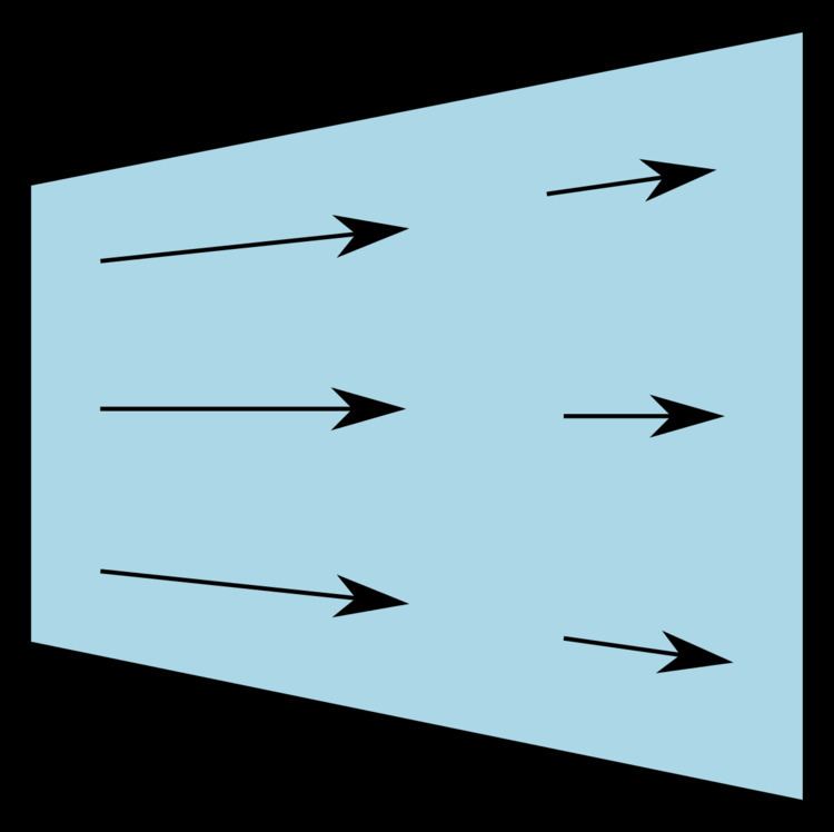
A significant feature of the Navier–Stokes equations is the presence of convective acceleration: the effect of time-independent acceleration of a flow with respect to space. While individual continuum particles indeed experience time dependent-acceleration, the convective acceleration of the flow field is a spatial effect, one example being fluid speeding up in a nozzle.

Regardless of what kind of continuum is being dealt with, convective acceleration is a nonlinear effect. Convective acceleration is present in most flows (exceptions include one-dimensional incompressible flow), but its dynamic effect is disregarded in creeping flow (also called Stokes flow). Convective acceleration is represented by the nonlinear quantity u · ∇u, which may be interpreted either as (u · ∇)u or as u · (∇u), with ∇u the tensor derivative of the velocity vector u. Both interpretations give the same result, independent of the coordinate system — provided ∇ is interpreted as the covariant derivative.

Advection operator

The convection term is often written as (u · ∇)u, where the advection operator u · ∇ is used. Usually this representation is preferred as it is simpler than the one in terms of the tensor derivative ∇u.

Tensor derivative

Here ∇u is the tensor derivative of the velocity vector, equal in Cartesian coordinates to the component-by-component gradient. Note that the gradient of a vector is being defined as [∇u]_mi = ∂_m v_i, so that

[ u ⋅ ( ∇ u ) ] i = v m ∂ m v i = [ ( u ⋅ ∇ ) u ] i .

Lamb form

The vector calculus identity of the cross product of a curl holds:

v × ( ∇ × a ) = ∇ a ( v ⋅ a ) − v ⋅ ∇ a

where the Feynman subscript notation ∇_a is used, which means the subscripted gradient operates only on the factor a.

Lamb in his famous classical book Hydrodynamics (1895), still in print, used this identity to change the convective term of the flow velocity in rotational form, i.e. without a tensor derivative:

u ⋅ ∇ u = ∇ ( ∥ u ∥ 2 2 ) + ( ∇ × u ) × u .

the Cauchy momentum equation becomes:

∂ u ∂ t + 1 2 ∇ ( u 2 ) + ( ∇ × u ) × u = 1 ρ ∇ ⋅ σ + g

And basing on the other identity:

∇ ⋅ ( σ ρ ) = 1 ρ ∇ ⋅ σ − 1 ρ 2 σ ⋅ ∇ ρ

the Cauchy equation becomes:

∇ ⋅ ( 1 2 u 2 + σ ρ ) − g = 1 ρ 2 σ ⋅ ∇ ρ + u × ( ∇ × u ) − ∂ u ∂ t

In fact, in case of an external conservative field, by defining its potential φ:

∇ ⋅ ( 1 2 u 2 + ϕ + σ ρ ) = 1 ρ 2 σ ⋅ ∇ ρ + u × ( ∇ × u ) − ∂ u ∂ t

In case of a steady flow the time derivative of the flow velocity disappears, so the momentum equation becomes:

∇ ⋅ ( 1 2 u 2 + ϕ + σ ρ ) = 1 ρ 2 σ ⋅ ∇ ρ + u × ( ∇ × u )

And by projecting the momentum equation on the flow direction, i.e. along a streamline, the cross product disappears due to a vector calculus identity of the triple scalar product:

u ⋅ ∇ ⋅ ( 1 2 u 2 + ϕ + σ ρ ) = 1 ρ 2 u ⋅ ( σ ⋅ ∇ ρ )

In the steady incompressible case the mass equation is simply:

u ⋅ ∇ ρ = 0 ,

that is, the mass conservation for a steady incompressible flow states that the density along a streamline is constant.

In the Euler momentum equation in the steady incompressible case:

u ⋅ ∇ ⋅ ( 1 2 u 2 + ϕ + p ρ ) = p ρ 2 u ⋅ ∇ ρ

This leads to a considerable simplification:

u ⋅ ∇ ( 1 2 u 2 + ϕ + p ρ ) = 0

The convenience of defining the total head for an inviscid liquid flow is now apparent:

b l ≡ 1 2 u 2 + ϕ + p ρ ,

in fact, the above equation can be simply written as:

u ⋅ ∇ b l = 0

That is, the momentum balance for a steady inviscid and incompressible flow in an external conservative field states that the total head along a streamline is constant.

Irrotational flows

The Lamb form has use in irrotational flow, where the curl of the velocity (called vorticity) ω = ∇ × u is equal to zero. Therefore, this reduces to only

u ⋅ ∇ u = ∇ ( ∥ u ∥ 2 2 ) .

Stresses

The effect of stress in the continuum flow is represented by the ∇p and ∇ · τ terms; these are gradients of surface forces, analogous to stresses in a solid. Here ∇p is called the pressure gradient and arises from the isotropic part of the Cauchy stress tensor, which has order two. This part is given by normal stresses that turn up in almost all situations, dynamic or not. The anisotropic part of the stress tensor gives rise to ∇ · τ, which conventionally describes viscous forces; for incompressible flow, this is only a shear effect. Thus, τ is the deviatoric stress tensor, and the stress tensor is equal to:

σ = − p 1 + τ

where 1 is the identity matrix in the space considered and τ the shear tensor.

All non-relativistic momentum conservation equations, such as the Navier–Stokes equation, can be derived by beginning with the Cauchy momentum equation and specifying the stress tensor through a constitutive relation. By expressing the shear tensor in terms of viscosity and fluid velocity, and assuming constant density and viscosity, the Cauchy momentum equation will lead to the Navier–Stokes equations. By assuming inviscid flow, the Navier–Stokes equations can further simplify to the Euler equations.

The divergence of the stress tensor can be written as

∇ ⋅ σ = − ∇ p + ∇ ⋅ τ .

The effect of the pressure gradient on the flow is to accelerate the flow in the direction from high pressure to low pressure.

The stress terms p and τ are yet unknown, so the general form of the equations of motion is not usable to solve problems. Besides the equations of motion—Newton's second law—a force model is needed relating the stresses to the flow motion. For this reason, assumptions based on natural observations are often applied to specify the stresses in terms of the other flow variables, such as velocity and density.

Nondimensionalisation

In order to make the equations dimensionless, a characteristic length r₀ and a characteristic velocity u₀ need to be defined. These should be chosen such that the dimensionless variables are all of order one. The following dimensionless variables are thus obtained:

ρ ∗ ≡ ρ ρ 0 u ∗ ≡ u u 0 r ∗ ≡ r r 0 t ∗ ≡ u 0 r 0 t ∇ ∗ ≡ r 0 ∇ g ∗ ≡ g g 0 p ∗ ≡ p p 0 τ ∗ ≡ τ τ 0

Substitution of these inverted relations in the Euler momentum equations yields:

ρ 0 u 0 2 r 0 ∂ ρ ∗ u ∗ ∂ t ∗ + ∇ ∗ r 0 ⋅ ( ρ 0 u 0 2 ρ ∗ u ∗ ⊗ u ∗ + p 0 p ∗ ) = − τ 0 r 0 ∇ ∗ ⋅ τ ∗ + g 0 g ∗

and by dividing for the first coefficient:

∂ ρ ∗ u ∗ ∂ t ∗ + ∇ ∗ ⋅ ( ρ ∗ u ∗ ⊗ u ∗ + p 0 ρ 0 u 0 2 p ∗ ) = − τ 0 ρ 0 u 0 2 ∇ ∗ ⋅ τ ∗ + g 0 r 0 u 0 2 g ∗

Now defining the Froude number:

F r = u 0 2 g 0 r 0 ,

the Euler number:

E u = p 0 ρ 0 u 0 2 ,

and the coefficient of frication:

C f = 2 τ 0 ρ 0 u 0 2 ,

by passing respectively to the conservative variables, i.e. the momentum density and the force density:

j = ρ u f = ρ g

the equations are finally expressed (now omitting the indexes):

Cauchy equations in the Froude limit Fr → ∞ (corresponding to negligible external field) are named free Cauchy equations:

and can be eventually conservation equations. The limit of high Froude numbers (low external field) is thus notable for such equations and is studied with perturbation theory.

Finally in convective form the equations are:

Cartesian 3D coordinates

x : ∂ u x ∂ t + u x ∂ u x ∂ x + u y ∂ u x ∂ y + u z ∂ u x ∂ z = 1 ρ ( − ∂ P ∂ x + ∂ τ x x ∂ x + ∂ τ x y ∂ y + ∂ τ x z ∂ z ) + g x y : ∂ u y ∂ t + u x ∂ u y ∂ x + u y ∂ u y ∂ y + u z ∂ u y ∂ z = 1 ρ ( − ∂ P ∂ y + ∂ τ y x ∂ x + ∂ τ y y ∂ y + ∂ τ y z ∂ z ) + g y z : ∂ u z ∂ t + u x ∂ u z ∂ x + u y ∂ u z ∂ y + u z ∂ u z ∂ z = 1 ρ ( − ∂ P ∂ z + ∂ τ z x ∂ x + ∂ τ z y ∂ y + ∂ τ z z ∂ z ) + g z

Cylindrical 3D coordinates

r : ∂ u r ∂ t + u r ∂ u r ∂ r + u ϕ r ∂ u r ∂ ϕ + u z ∂ u r ∂ z − u ϕ 2 r = − 1 ρ ∂ P ∂ r + 1 r ρ ∂ ( r τ r r ) ∂ r + 1 r ρ ∂ τ ϕ r ∂ ϕ + 1 ρ ∂ τ z r ∂ z − τ ϕ ϕ r ρ + g r ϕ : ∂ u ϕ ∂ t + u r ∂ u ϕ ∂ r + u ϕ r ∂ u ϕ ∂ ϕ + u z ∂ u ϕ ∂ z + u r u ϕ r = − 1 r ρ ∂ P ∂ ϕ + 1 r ρ ∂ τ ϕ ϕ ∂ ϕ + 1 r 2 ρ ∂ ( r 2 τ r ϕ ) ∂ r + 1 ρ ∂ τ z ϕ ∂ z + g ϕ z : ∂ u z ∂ t + u r ∂ u z ∂ r + u ϕ r ∂ u z ∂ ϕ + u z ∂ u z ∂ z = − 1 ρ ∂ P ∂ z + 1 ρ ∂ τ z z ∂ z + 1 r ρ ∂ τ ϕ z ∂ ϕ + 1 r ρ ∂ ( r τ r z ) ∂ r + g z

References

Cauchy momentum equation Wikipedia

(Text) CC BY-SA

Contents