Decision tree learning

General

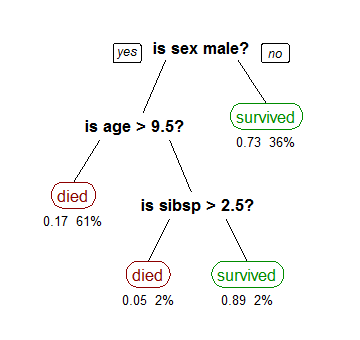
Decision tree learning is a method commonly used in data mining. The goal is to create a model that predicts the value of a target variable based on several input variables. An example is shown in the diagram at right. Each interior node corresponds to one of the input variables; there are edges to children for each of the possible values of that input variable. Each leaf represents a value of the target variable given the values of the input variables represented by the path from the root to the leaf.

A decision tree is a simple representation for classifying examples. For this section, assume that all of the input features have finite discrete domains, and there is a single target feature called the classification. Each element of the domain of the classification is called a class. A decision tree or a classification tree is a tree in which each internal (non-leaf) node is labeled with an input feature. The arcs coming from a node labeled with an input feature are labeled with each of the possible values of the target or output feature or the arc leads to a subordinate decision node on a different input feature. Each leaf of the tree is labeled with a class or a probability distribution over the classes.

A tree can be "learned" by splitting the source set into subsets based on an attribute value test. This process is repeated on each derived subset in a recursive manner called recursive partitioning. See the examples illustrated in the figure for spaces that have and have not been partitioned using recursive partitioning, or recursive binary splitting. The recursion is completed when the subset at a node has all the same value of the target variable, or when splitting no longer adds value to the predictions. This process of top-down induction of decision trees (TDIDT) is an example of a greedy algorithm, and it is by far the most common strategy for learning decision trees from data.

In data mining, decision trees can be described also as the combination of mathematical and computational techniques to aid the description, categorization and generalization of a given set of data.

Data comes in records of the form:

( x , Y ) = ( x 1 , x 2 , x 3 , . . . , x k , Y )

The dependent variable, Y, is the target variable that we are trying to understand, classify or generalize. The vector x is composed of the input variables, x₁, x₂, x₃ etc., that are used for that task.

Types

Decision trees used in data mining are of two main types:

Classification tree analysis is when the predicted outcome is the class to which the data belongs.

Regression tree analysis is when the predicted outcome can be considered a real number (e.g. the price of a house, or a patient's length of stay in a hospital).

The term Classification And Regression Tree (CART) analysis is an umbrella term used to refer to both of the above procedures, first introduced by Breiman et al. Trees used for regression and trees used for classification have some similarities - but also some differences, such as the procedure used to determine where to split.

Some techniques, often called ensemble methods, construct more than one decision tree:

Bagging decision trees, an early ensemble method, builds multiple decision trees by repeatedly resampling training data with replacement, and voting the trees for a consensus prediction.

A Random Forest classifier uses a number of decision trees in order to improve the classification rate.

Boosted Trees can be used for regression-type and classification-type problems.

Rotation forest - in which every decision tree is trained by first applying principal component analysis (PCA) on a random subset of the input features.

A special case of a decision tree is a Decision list, which is a one-sided decision tree, so that every internal node has exactly 1 leaf node and exactly 1 internal node as a child (except for the bottommost node, whose only child is a single leaf node). While less expressive, decision lists are arguably easier to understand than general decision trees due to their added sparsity, permit non-greedy learning methods and monotonic constraints to be imposed.

Decision tree learning is the construction of a decision tree from class-labeled training tuples. A decision tree is a flow-chart-like structure, where each internal (non-leaf) node denotes a test on an attribute, each branch represents the outcome of a test, and each leaf (or terminal) node holds a class label. The topmost node in a tree is the root node.

There are many specific decision-tree algorithms. Notable ones include:

ID3 (Iterative Dichotomiser 3)

C4.5 (successor of ID3)

CART (Classification And Regression Tree)

CHAID (CHi-squared Automatic Interaction Detector). Performs multi-level splits when computing classification trees.

MARS: extends decision trees to handle numerical data better.

Conditional Inference Trees. Statistics-based approach that uses non-parametric tests as splitting criteria, corrected for multiple testing to avoid overfitting. This approach results in unbiased predictor selection and does not require pruning.

ID3 and CART were invented independently at around the same time (between 1970 and 1980), yet follow a similar approach for learning decision tree from training tuples.

Metrics

Algorithms for constructing decision trees usually work top-down, by choosing a variable at each step that best splits the set of items. Different algorithms use different metrics for measuring "best". These generally measure the homogeneity of the target variable within the subsets. Some examples are given below. These metrics are applied to each candidate subset, and the resulting values are combined (e.g., averaged) to provide a measure of the quality of the split.

Gini impurity

Used by the CART (classification and regression tree) algorithm, Gini impurity is a measure of how often a randomly chosen element from the set would be incorrectly labeled if it was randomly labeled according to the distribution of labels in the subset. Gini impurity can be computed by summing the probability f i of an item with label i being chosen times the probability 1 − f i of a mistake in categorizing that item. It reaches its minimum (zero) when all cases in the node fall into a single target category.

To compute Gini impurity for a set of items with J classes, suppose i ∈ { 1 , 2 , . . . , J } , and let f i be the fraction of items labeled with class i in the set.

I G ( f ) = ∑ i = 1 J f i ( 1 − f i ) = ∑ i = 1 J ( f i − f i 2 ) = ∑ i = 1 J f i − ∑ i = 1 J f i 2 = 1 − ∑ i = 1 J f i 2 = ∑ i ≠ k f i f k

Information gain

Used by the ID3, C4.5 and C5.0 tree-generation algorithms. Information gain is based on the concept of entropy from information theory.

Entropy is defined as below

H ( T ) = I E ( p 1 , p 2 , . . . , p n ) = − ∑ i = 1 J p i log 2 ⁡ p i where p 1 , p 2 , . . . are fractions that add up to 1 and represent the percentage of each class present in the child node that results from a split in the tree.

Information Gain = Entropy(parent) - Weighted Sum of Entropy(Children)

I G ( T , a ) = H ( T ) − H ( T | a )

Information gain is used to decide which feature to split on at each step in building the tree. Simplicity is best, so we want to keep our tree small. To do so, at each step we should choose the split that results in the purest daughter nodes. A commonly used measure of purity is called information which is measured in bits, not to be confused with the unit of computer memory. For each node of the tree, the information value "represents the expected amount of information that would be needed to specify whether a new instance should be classified yes or no, given that the example reached that node".

Consider an example data set with four attributes: outlook (sunny, overcast, rainy), temperature (hot, mild, cool), humidity (high, normal), and windy (true, false), with a binary (yes or no) target variable, play, and 14 data points. To construct a decision tree on this data, we need to compare the information gain of each of four trees, each split on one of the four features. The split with the highest information gain will be taken as the first split and the process will continue until all children nodes are pure, or until the information gain is 0.

The split using the feature windy results in two children nodes, one for a windy value of true and one for a windy value of false. In this data set, there are six data points with a true windy value, three of which have a play value of yes and three with a play value of no. The eight remaining data points with a windy value of false contain two no's and six yes's. The information of the windy=true node is calculated using the entropy equation above. Since there is an equal number of yes's and no's in this node, we have

I E ( [ 3 , 3 ] ) = − ( 3 / 6 ) log 2 ⁡ ( 3 / 6 ) − ( 3 / 6 ) log 2 ⁡ ( 3 / 6 ) = − ( 1 / 2 ) log 2 ⁡ ( 1 / 2 ) − ( 1 / 2 ) log 2 ⁡ ( 1 / 2 ) = 1

For the node where windy=false there were eight data points, six yes's and two no's. Thus we have

I E ( [ 6 , 2 ] ) = − ( 6 / 8 ) log 2 ⁡ ( 6 / 8 ) − ( 2 / 8 ) log 2 ⁡ ( 2 / 8 ) = − ( 3 / 4 ) log 2 ⁡ ( 3 / 4 ) − ( 1 / 4 ) log 2 ⁡ ( 1 / 4 ) = 0.8112781

To find the information of the split, we take the weighted average of these two numbers based on how many observations fell into which node.

I E ( [ 3 , 3 ] , [ 6 , 2 ] ) = I E ( w i n d y o r n o t ) = ( 6 / 14 ) ( 1 ) + ( 8 / 14 ) ( 0.8112781 ) = 0.8921589

To find the information gain of the split using windy, we must first calculate the information in the data before the split. The original data contained nine yes's and five no's.

I E ( [ 9 , 5 ] ) = − ( 9 / 14 ) log 2 ⁡ ( 9 / 14 ) − ( 5 / 14 ) log 2 ⁡ ( 5 / 14 ) = 0.940286

Now we can calculate the information gain achieved by splitting on the windy feature.

I G ( w i n d y ) = I E ( [ 9 , 5 ] ) − I E ( [ 3 , 3 ] , [ 6 , 2 ] ) = 0.940286 − 0.8921589 = 0.0481271

To build the tree, the information gain of each possible first split would need to be calculated. The best first split is the one that provides the most information gain. This process is repeated for each impure node until the tree is complete. This example is adapted from the example appearing in Witten et al.

Variance reduction

Introduced in CART, variance reduction is often employed in cases where the target variable is continuous (regression tree), meaning that use of many other metrics would first require discretization before being applied. The variance reduction of a node N is defined as the total reduction of the variance of the target variable x due to the split at this node:

I V ( N ) = 1 | S | 2 ∑ i ∈ S ∑ j ∈ S 1 2 ( x i − x j ) 2 − ( 1 | S t | 2 ∑ i ∈ S t ∑ j ∈ S t 1 2 ( x i − x j ) 2 + 1 | S f | 2 ∑ i ∈ S f ∑ j ∈ S f 1 2 ( x i − x j ) 2 )

where S , S t , and S f are the set of presplit sample indices, set of sample indices for which the split test is true, and set of sample indices for which the split test is false, respectively. Each of the above summands are indeed variance estimates, though, written in a form without directly referring to the mean.

Decision tree advantages

Amongst other data mining methods, decision trees have various advantages:

Simple to understand and interpret. People are able to understand decision tree models after a brief explanation. Trees can also be displayed graphically in a way that is easy for non-experts to interpret.

Able to handle both numerical and categorical data. Other techniques are usually specialised in analysing datasets that have only one type of variable. (For example, relation rules can be used only with nominal variables while neural networks can be used only with numerical variables.)

Requires little data preparation. Other techniques often require data normalization. Since trees can handle qualitative predictors, there is no need to create dummy variables.

Uses a white box model. If a given situation is observable in a model the explanation for the condition is easily explained by boolean logic. By contrast, in a black box model, the explanation for the results is typically difficult to understand, for example with an artificial neural network.

Possible to validate a model using statistical tests. That makes it possible to account for the reliability of the model.

Robust. Performs well even if its assumptions are somewhat violated by the true model from which the data were generated.

Performs well with large datasets. Large amounts of data can be analysed using standard computing resources in reasonable time.

Mirrors human decision making more closely than other approaches. This could be useful when modeling human decisions/behavior.

Limitations

Trees do not tend to be as accurate as other approaches.

Trees can be very non-robust. A small change in the training data can result in a big change in the tree, and thus a big change in final predictions.

The problem of learning an optimal decision tree is known to be NP-complete under several aspects of optimality and even for simple concepts. Consequently, practical decision-tree learning algorithms are based on heuristics such as the greedy algorithm where locally-optimal decisions are made at each node. Such algorithms cannot guarantee to return the globally-optimal decision tree. To reduce the greedy effect of local-optimality some methods such as the dual information distance (DID) tree were proposed. [1]

Decision-tree learners can create over-complex trees that do not generalize well from the training data. (This is known as overfitting.) Mechanisms such as pruning are necessary to avoid this problem (with the exception of some algorithms such as the Conditional Inference approach, that does not require pruning ).

There are concepts that are hard to learn because decision trees do not express them easily, such as XOR, parity or multiplexer problems. In such cases, the decision tree becomes prohibitively large. Approaches to solve the problem involve either changing the representation of the problem domain (known as propositionalization) or using learning algorithms based on more expressive representations (such as statistical relational learning or inductive logic programming).

For data including categorical variables with different numbers of levels, information gain in decision trees is biased in favor of those attributes with more levels. However, the issue of biased predictor selection is avoided by the Conditional Inference approach.

Decision graphs

In a decision tree, all paths from the root node to the leaf node proceed by way of conjunction, or AND. In a decision graph, it is possible to use disjunctions (ORs) to join two more paths together using Minimum message length (MML). Decision graphs have been further extended to allow for previously unstated new attributes to be learnt dynamically and used at different places within the graph. The more general coding scheme results in better predictive accuracy and log-loss probabilistic scoring. In general, decision graphs infer models with fewer leaves than decision trees.

Alternative search methods

Evolutionary algorithms have been used to avoid local optimal decisions and search the decision tree space with little a priori bias.

It is also possible for a tree to be sampled using MCMC.

The tree can be searched for in a bottom-up fashion.

Implementations

Many data mining software packages provide implementations of one or more decision tree algorithms. Several examples include Salford Systems CART (which licensed the proprietary code of the original CART authors), IBM SPSS Modeler, RapidMiner, SAS Enterprise Miner, Matlab, R (an open source software environment for statistical computing which includes several CART implementations such as rpart, party and randomForest packages), Weka (a free and open-source data mining suite, contains many decision tree algorithms), Orange (a free data mining software suite, which includes the tree module orngTree), KNIME, Microsoft SQL Server [2], and scikit-learn (a free and open-source machine learning library for the Python programming language).