Odds ratio

A motivating example, in the context of the rare disease assumption

Imagine there is a rare disease, afflicting, say, only one in many thousands of adults in a country. Imagine we suspect that being exposed to something (say, having had a particular sort of injury in childhood) makes one more likely to develop that disease in adulthood. The most informative thing to compute would be the risk ratio, RR. To do this in the ideal case, for all the adults in the population we would need to know whether they (a) had the exposure to the injury as children and (b) whether they developed the disease as adults. From this we would extract the following information: the total number of people exposed to the childhood injury, N E , out of which D E developed the disease and H E stayed healthy; and the total number of people not exposed, N N , out of which D N developed the disease and H N stayed healthy. Since N E = D E + H E and similarly for the N N numbers, we only have four independent numbers, which we can organize in a table:

To avoid possible confusion, we emphasize that all these numbers refer to the entire population, and not to some sample of it.

Now the risk of developing the disease given exposure is D E / N E (where N E = D E + H E ), and of developing the disease given non-exposure is D N / N N . The risk ratio, RR, is just the ratio of the two,

which can be rewritten as R R = D E N N D N N E = D E / D N N E / N N .

In contrast, the odds of developing the disease given exposure is D E / H E , and of developing the disease given non-exposure is D N / H N . The odds ratio, OR, is the ratio of the two,

which can be rewritten as O R = D E H N D N H E = D E / D N H E / H N .

We may already note that if the disease is rare, then OR ≈ RR. Indeed, for a rare disease, we will have D E ≪ H E , and so D E + H E ≈ H E ; but then D E / ( D E + H E ) ≈ D E / H E , in other words, for the exposed population, the risk of developing the disease is approximately equal to the odds. Analogous reasoning shows that the risk is approximately equal to the odds for the non-exposed population as well; but then the ratio of the risks, which is RR, is approximately equal to the ratio of the odds, which is OR. Or, we could just notice that the rare disease assumption says that N E ≈ H E and N N ≈ H N , from which it follows that N E / N N ≈ H E / H N , in other words that the denominators in the final expressions for the RR and the OR are approximately the same. The numerators are exactly the same, and so, again, we conclude that OR ≈ RR. Returning to our hypothetical study, the problem we often face is that we may not have the data to estimate these four numbers. For example, we may not have the population-wide data on who did or did not have the childhood injury.

Often we may overcome this problem by employing random sampling of the population: namely, if neither the disease nor the exposure to the injury are too rare in our population, then we can pick (say) a hundred people at random, and find out these four numbers in that sample; assuming the sample is representative enough of the population, then the RR computed for this sample will be a good estimate for the RR for the whole population.

However, some diseases may be so rare that, in all likelihood, even a large random sample may not contain even a single diseased individual (or it may contain some, but too few to be statistically significant). This would make it impossible to compute the RR. But, we may nevertheless be able to estimate the OR, provided that, unlike the disease, the exposure to the childhood injury is not too rare. Of course, because the disease is rare, this is then also our estimate for the RR.

Looking at the final expression for the OR: the fraction in the numerator, D E / D N , we can estimate by collecting all the known cases of the disease (presumably there must be some, or else we likely wouldn't be doing the study in the first place), and seeing how many of the diseased people had the exposure, and how many did not. And the fraction in the denominator, H E / H N , is the odds that a healthy individual in the population was exposed to the childhood injury. Now note that this latter odds can indeed be estimated by random sampling of the population—provided, as we said, that the prevalence of the exposure to the childhood injury is not too small, so that a random sample of a manageable size would be likely to contain a fair number of individuals who have had the exposure. So here the disease is very rare, but the factor thought to contribute to it is not quite so rare; such situations are quite common in practice.

Thus we can estimate the OR, and then, invoking the rare disease assumption again, we say that this is also a good approximation of the RR. Incidentally, the story just told is a paradigmatic example of a case-control study.

The same story could be told without ever mentioning the OR, like so: as soon as we have that N E ≈ H E and N N ≈ H N , then we have that N E / N N ≈ H E / H N . Thus if, by random sampling, we manage to estimate H E / H N , then, by rare disease assumption, that will be a good estimate of N E / N N , which is all we need (besides D E / D N , which we presumably already know by studying the few cases of the disease) to compute the RR. However, it is standard in the literature to explicitly report the OR and then claim that the RR is approximately equal to it.

Definition in terms of group-wise odds

The odds ratio is the ratio of the odds of an event occurring in one group to the odds of it occurring in another group. The term is also used to refer to sample-based estimates of this ratio. These groups might be men and women, an experimental group and a control group, or any other dichotomous classification. If the probabilities of the event in each of the groups are p₁ (first group) and p₂ (second group), then the odds ratio is:

where q_x = 1 − p_x. An odds ratio of 1 indicates that the condition or event under study is equally likely to occur in both groups. An odds ratio greater than 1 indicates that the condition or event is more likely to occur in the first group. And an odds ratio less than 1 indicates that the condition or event is less likely to occur in the first group. The odds ratio must be nonnegative if it is defined. It is undefined if p₂q₁ equals zero, i.e., if p₂ equals zero or q₁ equals zero.

Definition in terms of joint and conditional probabilities

The odds ratio can also be defined in terms of the joint probability distribution of two binary random variables. The joint distribution of binary random variables X and Y can be written

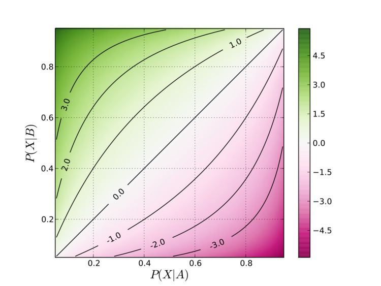
where p₁₁, p₁₀, p₀₁ and p₀₀ are non-negative "cell probabilities" that sum to one. The odds for Y within the two subpopulations defined by X = 1 and X = 0 are defined in terms of the conditional probabilities given X, i.e., P(Y|X):

Thus the odds ratio is

The simple expression on the right, above, is easy to remember as the product of the probabilities of the "concordant cells" (X = Y) divided by the product of the probabilities of the "discordant cells" (X ≠ Y). However note that in some applications the labeling of categories as zero and one is arbitrary, so there is nothing special about concordant versus discordant values in these applications.

Symmetry

If we had calculated the odds ratio based on the conditional probabilities given Y,

we would have gotten the same result

Other measures of effect size for binary data such as the relative risk do not have this symmetry property.

Relation to statistical independence

If X and Y are independent, their joint probabilities can be expressed in terms of their marginal probabilities p_x =  P(X = 1) and p_y =  P(Y = 1), as follows

In this case, the odds ratio equals one, and conversely the odds ratio can only equal one if the joint probabilities can be factored in this way. Thus the odds ratio equals one if and only if X and Y are independent.

Recovering the cell probabilities from the odds ratio and marginal probabilities

The odds ratio is a function of the cell probabilities, and conversely, the cell probabilities can be recovered given knowledge of the odds ratio and the marginal probabilities P(X = 1) = p₁₁ + p₁₀ and P(Y = 1) = p₁₁ + p₀₁. If the odds ratio R differs from 1, then

where p_1• = p₁₁ + p₁₀,  p_•1 = p₁₁ + p₀₁, and

In the case where R = 1, we have independence, so p₁₁ = p_1•p_•1.

Once we have p₁₁, the other three cell probabilities can easily be recovered from the marginal probabilities.

Example

Suppose that in a sample of 100 men, 90 drank wine in the previous week, while in a sample of 100 women only 20 drank wine in the same period. The odds of a man drinking wine are 90 to 10, or 9:1, while the odds of a woman drinking wine are only 20 to 80, or 1:4 = 0.25:1. The odds ratio is thus 9/0.25, or 36, showing that men are much more likely to drink wine than women. The detailed calculation is:

This example also shows how odds ratios are sometimes sensitive in stating relative positions: in this sample men are 90/20 = 4.5 times as likely to have drunk wine than women, but have 36 times the odds. The logarithm of the odds ratio, the difference of the logits of the probabilities, tempers this effect, and also makes the measure symmetric with respect to the ordering of groups. For example, using natural logarithms, an odds ratio of 36/1 maps to 3.584, and an odds ratio of 1/36 maps to −3.584.

Statistical inference

Several approaches to statistical inference for odds ratios have been developed.

One approach to inference uses large sample approximations to the sampling distribution of the log odds ratio (the natural logarithm of the odds ratio). If we use the joint probability notation defined above, the population log odds ratio is

If we observe data in the form of a contingency table

then the probabilities in the joint distribution can be estimated as

where ︿p_ij = n_ij / n, with n = n₁₁ + n₁₀ + n₀₁ + n₀₀ being the sum of all four cell counts. The sample log odds ratio is

The distribution of the log odds ratio is approximately normal with:

The standard error for the log odds ratio is approximately

This is an asymptotic approximation, and will not give a meaningful result if any of the cell counts are very small. If L is the sample log odds ratio, an approximate 95% confidence interval for the population log odds ratio is L ± 1.96SE. This can be mapped to exp(L − 1.96SE), exp(L + 1.96SE) to obtain a 95% confidence interval for the odds ratio. If we wish to test the hypothesis that the population odds ratio equals one, the two-sided p-value is 2P(Z < −| L |/SE), where P denotes a probability, and Z denotes a standard normal random variable.

An alternative approach to inference for odds ratios looks at the distribution of the data conditionally on the marginal frequencies of X and Y. An advantage of this approach is that the sampling distribution of the odds ratio can be expressed exactly.

Role in logistic regression

Logistic regression is one way to generalize the odds ratio beyond two binary variables. Suppose we have a binary response variable Y and a binary predictor variable X, and in addition we have other predictor variables Z₁, ..., Z_p that may or may not be binary. If we use multiple logistic regression to regress Y on X, Z₁, ..., Z_p, then the estimated coefficient β ^ x for X is related to a conditional odds ratio. Specifically, at the population level

so exp ⁡ ( β ^ x ) is an estimate of this conditional odds ratio. The interpretation of exp ⁡ ( β ^ x ) is as an estimate of the odds ratio between Y and X when the values of Z₁, ..., Z_p are held fixed.

Insensitivity to the type of sampling

If the data form a "population sample", then the cell probabilities ∧p_ij are interpreted as the frequencies of each of the four groups in the population as defined by their X and Y values. In many settings it is impractical to obtain a population sample, so a selected sample is used. For example, we may choose to sample units with X = 1 with a given probability f, regardless of their frequency in the population (which would necessitate sampling units with X = 0 with probability 1 − f). In this situation, our data would follow the following joint probabilities:

The odds ratio p₁₁p₀₀ / p₀₁p₁₀ for this distribution does not depend on the value of f. This shows that the odds ratio (and consequently the log odds ratio) is invariant to non-random sampling based on one of the variables being studied. Note however that the standard error of the log odds ratio does depend on the value of f.

This fact is exploited in two important situations:

In both these settings, the odds ratio can be calculated from the selected sample, without biasing the results relative to what would have been obtained for a population sample.

Use in quantitative research

Due to the widespread use of logistic regression, the odds ratio is widely used in many fields of medical and social science research. The odds ratio is commonly used in survey research, in epidemiology, and to express the results of some clinical trials, such as in case-control studies. It is often abbreviated "OR" in reports. When data from multiple surveys is combined, it will often be expressed as "pooled OR".

Relation to relative risk

In clinical studies, as well as in some other settings, the parameter of greatest interest is often the relative risk rather than the odds ratio. The relative risk is best estimated using a population sample, but if the rare disease assumption holds, the odds ratio is a good approximation to the relative risk — the odds is p / (1 − p), so when p moves towards zero, 1 − p moves towards 1, meaning that the odds approaches the risk, and the odds ratio approaches the relative risk. When the rare disease assumption does not hold, the odds ratio can overestimate the relative risk.

If the absolute risk in the control group is available, conversion between the two is calculated by:

where:

Confusion and exaggeration

Odds ratios have often been confused with relative risk in medical literature. For non-statisticians, the odds ratio is a difficult concept to comprehend, and it gives a more impressive figure for the effect. However, most authors consider that the relative risk is readily understood. In one study, members of a national disease foundation were actually 3.5 times more likely than nonmembers to have heard of a common treatment for that disease – but the odds ratio was 24 and the paper stated that members were ‘more than 20-fold more likely to have heard of’ the treatment. A study of papers published in two journals reported that 26% of the articles that used an odds ratio interpreted it as a risk ratio.

This may reflect the simple process of uncomprehending authors choosing the most impressive-looking and publishable figure. But its use may in some cases be deliberately deceptive. It has been suggested that the odds ratio should only be presented as a measure of effect size when the risk ratio cannot be estimated directly.

Invertibility and invariance

The odds ratio has another unique property of being directly mathematically invertible whether analyzing the OR as either disease survival or disease onset incidence – where the OR for survival is direct reciprocal of 1/OR for risk. This is known as the 'invariance of the odds ratio'. In contrast, the relative risk does not possess this mathematical invertible property when studying disease survival vs. onset incidence. This phenomenon of OR invertibility vs. RR non-invertibility is best illustrated with an example:

Suppose in a clinical trial, one has an adverse event risk of 4/100 in drug group, and 2/100 in placebo... yielding a RR=2 and OR=2.04166 for drug-vs-placebo adverse risk. However, if analysis was inverted and adverse events were instead analyzed as event-free survival, then the drug group would have a rate of 96/100, and placebo group would have a rate of 98/100—yielding a drug-vs-placebo a RR=0.9796 for survival, but an OR=0.48979. As one can see, a RR of 0.9796 is clearly not the reciprocal of a RR of 2. In contrast, an OR of 0.48979 is indeed the direct reciprocal of an OR of 2.04166.

This is again what is called the 'invariance of the odds ratio', and why a RR for survival is not the same as a RR for risk, while the OR has this symmetrical property when analyzing either survival or adverse risk. The danger to clinical interpretation for the OR comes when the adverse event rate is not rare, thereby exaggerating differences when the OR rare-disease assumption is not met. On the other hand, when the disease is rare, using a RR for survival (e.g. the RR=0.9796 from above example) can clinically hide and conceal an important doubling of adverse risk associated with a drug or exposure.

Alternative estimators of the odds ratio

The sample odds ratio n₁₁n₀₀ / n₁₀n₀₁ is easy to calculate, and for moderate and large samples performs well as an estimator of the population odds ratio. When one or more of the cells in the contingency table can have a small value, the sample odds ratio can be biased and exhibit high variance. A number of alternative estimators of the odds ratio have been proposed to address this issue. One alternative estimator is the conditional maximum likelihood estimator, which conditions on the row and column margins when forming the likelihood to maximize (as in Fisher's exact test). Another alternative estimator is the Mantel-Haenszel estimator.

Numerical examples

The following four contingency tables contain observed cell counts, along with the corresponding sample odds ratio (OR) and sample log odds ratio (LOR):

The following joint probability distributions contain the population cell probabilities, along with the corresponding population odds ratio (OR) and population log odds ratio (LOR):