Law of large numbers

Examples

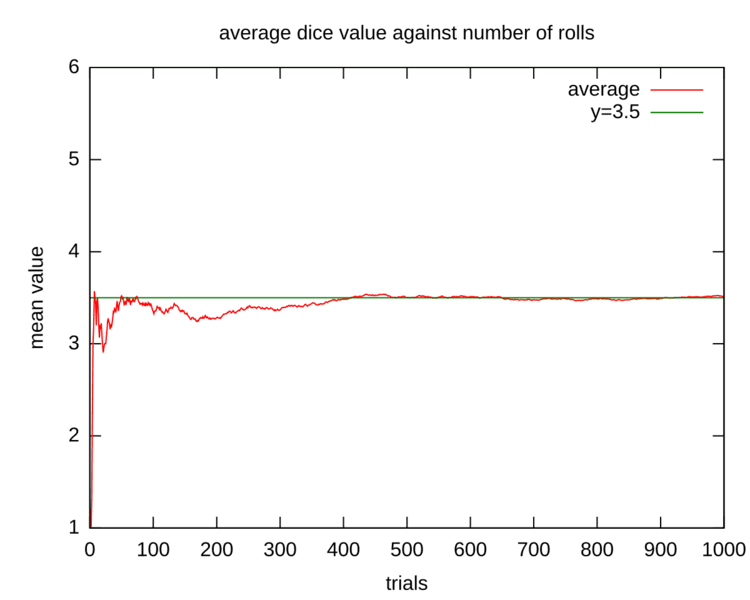
For example, a single roll of a fair, six-sided die produces one of the numbers 1, 2, 3, 4, 5, or 6, each with equal probability. Therefore, the expected value of a single die roll is

1 + 2 + 3 + 4 + 5 + 6 6 = 3.5

According to the law of large numbers, if a large number of six-sided dice are rolled, the average of their values (sometimes called the sample mean) is likely to be close to 3.5, with the precision increasing as more dice are rolled.

It follows from the law of large numbers that the empirical probability of success in a series of Bernoulli trials will converge to the theoretical probability. For a Bernoulli random variable, the expected value is the theoretical probability of success, and the average of n such variables (assuming they are independent and identically distributed (i.i.d.)) is precisely the relative frequency.

For example, a fair coin toss is a Bernoulli trial. When a fair coin is flipped once, the theoretical probability that the outcome will be heads is equal to 1/2. Therefore, according to the law of large numbers, the proportion of heads in a "large" number of coin flips "should be" roughly 1/2. In particular, the proportion of heads after n flips will almost surely converge to 1/2 as n approaches infinity.

Though the proportion of heads (and tails) approaches 1/2, almost surely the absolute difference in the number of heads and tails will become large as the number of flips becomes large. That is, the probability that the absolute difference is a small number, approaches zero as the number of flips becomes large. Also, almost surely the ratio of the absolute difference to the number of flips will approach zero. Intuitively, expected absolute difference grows, but at a slower rate than the number of flips, as the number of flips grows.

History

The Italian mathematician Gerolamo Cardano (1501–1576) stated without proof that the accuracies of empirical statistics tend to improve with the number of trials. This was then formalized as a law of large numbers. A special form of the LLN (for a binary random variable) was first proved by Jacob Bernoulli. It took him over 20 years to develop a sufficiently rigorous mathematical proof which was published in his Ars Conjectandi (The Art of Conjecturing) in 1713. He named this his "Golden Theorem" but it became generally known as "Bernoulli's Theorem". This should not be confused with Bernoulli's principle, named after Jacob Bernoulli's nephew Daniel Bernoulli. In 1837, S.D. Poisson further described it under the name "la loi des grands nombres" ("The law of large numbers"). Thereafter, it was known under both names, but the "Law of large numbers" is most frequently used.

After Bernoulli and Poisson published their efforts, other mathematicians also contributed to refinement of the law, including Chebyshev, Markov, Borel, Cantelli and Kolmogorov and Khinchin. Markov showed that the law can apply to a random variable that does not have a finite variance under some other weaker assumption, and Khinchin showed in 1929 that if the series consists of independent identically distributed random variables, it suffices that the expected value exists for the weak law of large numbers to be true. These further studies have given rise to two prominent forms of the LLN. One is called the "weak" law and the other the "strong" law, in reference to two different modes of convergence of the cumulative sample means to the expected value; in particular, as explained below, the strong form implies the weak.

Forms

Two different versions of the law of large numbers are described below; they are called the strong law of large numbers, and the weak law of large numbers. Stated for the case where X₁, X₂, ... is an infinite sequence of i.i.d. Lebesgue integrable random variables with expected value E(X₁) = E(X₂) = ...= µ, both versions of the law state that – with virtual certainty – the sample average

X ¯ n = 1 n ( X 1 + ⋯ + X n )

converges to the expected value

(Lebesgue integrability of X_j means that the expected value E(X_j) exists according to Lebesgue integration and is finite.)

An assumption of finite variance Var(X₁) = Var(X₂) = ... = σ² < ∞ is not necessary. Large or infinite variance will make the convergence slower, but the LLN holds anyway. This assumption is often used because it makes the proofs easier and shorter.

The difference between the strong and the weak version is concerned with the mode of convergence being asserted. For interpretation of these modes, see Convergence of random variables.

Weak law

The weak law of large numbers (also called Khintchine's law) states that the sample average converges in probability towards the expected value

That is to say that for any positive number ε,

lim n → ∞ Pr ( | X ¯ n − μ | > ε ) = 0.

Interpreting this result, the weak law essentially states that for any nonzero margin specified, no matter how small, with a sufficiently large sample there will be a very high probability that the average of the observations will be close to the expected value; that is, within the margin.

Convergence in probability is also called weak convergence of random variables. This version is called the weak law because random variables may converge weakly (in probability) as above without converging strongly (almost surely) as below.

As mentioned earlier, the weak law applies in the case of independent identically distributed random variables having an expected value. But it also applies in some other cases. For example, the variance may be different for each random variable in the series, keeping the expected value constant. If the variances are bounded, then the law applies, as shown by Chebyshev as early as 1867. (If the expected values change during the series, then we can simply apply the law to the average deviation from the respective expected values. The law then states that this converges in probability to zero.) In fact, Chebyshev's proof works so long as the variance of the average of the first n values goes to zero as n goes to infinity. As an example, assume that each random variable in the series follows a Gaussian distribution with mean zero, but with variance equal to 2 n / log ⁡ ( n + 1 ) . At each stage, the average will be normally distributed (since it is the average of a set of normally distributed variables). The variance of the sum is equal to the sum of the variances, which is asymptotic to n 2 / log ⁡ n . The variance of the average is therefore asymptotic to 1 / log ⁡ n and goes to zero.

An example where the law of large numbers does not apply is the Cauchy distribution. Let the random numbers equal the tangent of an angle uniformly distributed between −90° and +90°. The median is zero, but the expected value does not exist, and indeed the average of n such variables has the same distribution as one such variable. It does not tend toward zero as n goes to infinity.

There are also examples of the weak law applying even though the expected value does not exist. See #Differences between the weak law and the strong law.

Strong law

The strong law of large numbers states that the sample average converges almost surely to the expected value

That is,

Pr ( lim n → ∞ X ¯ n = μ ) = 1.

What this means is that as the number of trials n goes to infinity, the probability that the average of the observations is equal to the expected value will be equal to one.

The proof is more complex than that of the weak law. This law justifies the intuitive interpretation of the expected value (for Lebesgue integration only) of a random variable when sampled repeatedly as the "long-term average".

Almost sure convergence is also called strong convergence of random variables. This version is called the strong law because random variables which converge strongly (almost surely) are guaranteed to converge weakly (in probability). The strong law implies the weak law but not vice versa, when the strong law conditions hold the variable converges both strongly (almost surely) and weakly (in probability). However the weak law may hold in conditions where the strong law does not hold and then the convergence is only weak (in probability).

To date it has not been possible to prove that the strong law conditions are the same as those of the weak law.

The strong law of large numbers can itself be seen as a special case of the pointwise ergodic theorem.

The strong law applies to independent identically distributed random variables having an expected value (like the weak law). This was proved by Kolmogorov in 1930. It can also apply in other cases. Kolmogorov also showed, in 1933, that if the variables are independent and identically distributed, then for the average to converge almost surely on something (this can be considered another statement of the strong law), it is necessary that they have an expected value (and then of course the average will converge almost surely on that).

If the summands are independent but not identically distributed, then

X ¯ n − E ⁡ [ X ¯ n ]   → a.s.   0 ,

provided that each X_k has a finite second moment and

∑ k = 1 ∞ 1 k 2 Var ⁡ [ X k ] < ∞ .

This statement is known as Kolmogorov's strong law, see e.g. Sen & Singer (1993, Theorem 2.3.10).

An example of a series where the weak law applies but not the strong law is when X_k is plus or minus k / log ⁡ log ⁡ log ⁡ k (starting at sufficiently large k so that the denominator is positive) with probability 1/2 for each. The variance of X_k is then k / log ⁡ log ⁡ log ⁡ k . Kolmogorov's strong law does not apply because the partial sum in his criterion up to k=n is asymptotic to log ⁡ n / log ⁡ log ⁡ log ⁡ n and this is unbounded.

If we replace the random variables with Gaussian variables having the same variances, namely k / log ⁡ log ⁡ log ⁡ k , then the average at any point will also be normally distributed. The width of the distribution of the average will tend toward zero (standard deviation asymptotic to 1 / 2 log ⁡ log ⁡ log ⁡ n ), but for a given ε, there is probability which does not go to zero with n that the average sometime after the nth trial will come back up to ε. Since this probability does not go to zero, it must have a positive lower bound p(ε), which means there is a probability of at least p(ε) that the average will attain ε after n trials. It will happen with probability p(ε)/2 before some m which depends on n. But even after m, there is still a probability of at least p(ε) that it will happen. (This seems to indicate that p(ε)=1 and the average will attain ε an infinite number of times.)

Differences between the weak law and the strong law

The weak law states that for a specified large n, the average X ¯ n is likely to be near μ. Thus, it leaves open the possibility that | X ¯ n − μ | > ε happens an infinite number of times, although at infrequent intervals. (Not necessarily | X ¯ n − μ | ≠ 0 for all n ).

The strong law shows that this almost surely will not occur. In particular, it implies that with probability 1, we have that for any ε > 0 the inequality | X ¯ n − μ | < ε holds for all large enough n.

The strong law does not hold in the following cases, but the weak law does.

1. Let x be an exponentially distributed random variable with parameter 1. The random variable sin ⁡ ( x ) e x x has no expected value according to Lebesgue integration, but using conditional convergence and interpreting the integral as a Dirichlet integral, which is an improper Riemann integral, we can say:

E ( sin ⁡ ( x ) e x x ) =   ∫ 0 ∞ sin ⁡ ( x ) e x x e − x d x = π 2

2. Let x be geometric distribution with probability 0.5. The random variable 2 x ( − 1 ) x x does not have an expected value in the conventional sense because the infinite series is not absolutely convergent, but using conditional convergence, we can say:

E ( 2 x ( − 1 ) x x ) =   ∑ 1 ∞ 2 x ( − 1 ) x x 2 − x = − ln ⁡ ( 2 )

3. If the cumulative distribution function of a random variable is

1 − F ( x ) = e 2 x ln ⁡ ( x ) , x ≥ e F ( x ) = e − 2 x ln ⁡ ( − x ) , x ≤ − e then it has no expected value, but the weak law is true.

Uniform law of large numbers

Suppose f(x,θ) is some function defined for θ ∈ Θ, and continuous in θ. Then for any fixed θ, the sequence {f(X₁,θ), f(X₂,θ), …} will be a sequence of independent and identically distributed random variables, such that the sample mean of this sequence converges in probability to E[f(X,θ)]. This is the pointwise (in θ) convergence.

The uniform law of large numbers states the conditions under which the convergence happens uniformly in θ. If

1. Θ is compact,
2. f(x,θ) is continuous at each θ ∈ Θ for almost all x’s, and measurable function of x at each θ.
3. there exists a dominating function d(x) such that E[d(X)] < ∞, and ∥ f ( x , θ ) ∥ ≤ d ( x ) for all   θ ∈ Θ .

Then E[f(X,θ)] is continuous in θ, and

sup θ ∈ Θ ∥ 1 n ∑ i = 1 n f ( X i , θ ) − E ⁡ [ f ( X , θ ) ] ∥ → a . s .   0.

This result is useful to derive consistency of a large class of estimators (see Extremum estimator).

Borel's law of large numbers

Borel's law of large numbers, named after Émile Borel, states that if an experiment is repeated a large number of times, independently under identical conditions, then the proportion of times that any specified event occurs approximately equals the probability of the event's occurrence on any particular trial; the larger the number of repetitions, the better the approximation tends to be. More precisely, if E denotes the event in question, p its probability of occurrence, and N_n(E) the number of times E occurs in the first n trials, then with probability one,

N n ( E ) n → p  as  n → ∞ .

Chebyshev's inequality. Let X be a random variable with finite expected value μ and finite non-zero variance σ². Then for any real number k > 0,

Pr ( | X − μ | ≥ k σ ) ≤ 1 k 2 .

This theorem makes rigorous the intuitive notion of probability as the long-run relative frequency of an event's occurrence. It is a special case of any of several more general laws of large numbers in probability theory.

Proof of the weak law

Given X₁, X₂, ... an infinite sequence of i.i.d. random variables with finite expected value E(X₁) = E(X₂) = ... = µ < ∞, we are interested in the convergence of the sample average

X ¯ n = 1 n ( X 1 + ⋯ + X n ) .

The weak law of large numbers states:

Proof using Chebyshev's inequality

This proof uses the assumption of finite variance Var ⁡ ( X i ) = σ 2 (for all i ). The independence of the random variables implies no correlation between them, and we have that

Var ⁡ ( X ¯ n ) = Var ⁡ ( 1 n ( X 1 + ⋯ + X n ) ) = 1 n 2 Var ⁡ ( X 1 + ⋯ + X n ) = n σ 2 n 2 = σ 2 n .

The common mean μ of the sequence is the mean of the sample average:

E ( X ¯ n ) = μ .

Using Chebyshev's inequality on X ¯ n results in

P ⁡ ( | X ¯ n − μ | ≥ ε ) ≤ σ 2 n ε 2 .

This may be used to obtain the following:

P ⁡ ( | X ¯ n − μ | < ε ) = 1 − P ⁡ ( | X ¯ n − μ | ≥ ε ) ≥ 1 − σ 2 n ε 2 .

As n approaches infinity, the expression approaches 1. And by definition of convergence in probability, we have obtained

Proof using convergence of characteristic functions

By Taylor's theorem for complex functions, the characteristic function of any random variable, X, with finite mean μ, can be written as

φ X ( t ) = 1 + i t μ + o ( t ) , t → 0.

All X₁, X₂, ... have the same characteristic function, so we will simply denote this φ_X.

Among the basic properties of characteristic functions there are

φ 1 n X ( t ) = φ X ( t n ) and φ X + Y ( t ) = φ X ( t ) φ Y ( t ) if X and Y are independent.

These rules can be used to calculate the characteristic function of X ¯ n in terms of φ_X:

φ X ¯ n ( t ) = [ φ X ( t n ) ] n = [ 1 + i μ t n + o ( t n ) ] n → e i t μ , as n → ∞ .

The limit  e^itμ  is the characteristic function of the constant random variable μ, and hence by the Lévy continuity theorem, X ¯ n converges in distribution to μ:

X ¯ n → D μ for n → ∞ .

μ is a constant, which implies that convergence in distribution to μ and convergence in probability to μ are equivalent (see Convergence of random variables.) Therefore,

This shows that the sample mean converges in probability to the derivative of the characteristic function at the origin, as long as the latter exists.