Mild slope equation - Alchetron, The Free Social Encyclopedia

In fluid dynamics, the mild-slope equation describes the combined effects of diffraction and refraction for water waves propagating over bathymetry and due to lateral boundaries—like breakwaters and coastlines. It is an approximate model, deriving its name from being originally developed for wave propagation over mild slopes of the sea floor. The mild-slope equation is often used in coastal engineering to compute the wave-field changes near harbours and coasts.

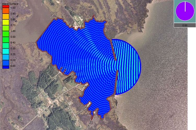
The mild-slope equation models the propagation and transformation of water waves, as they travel through waters of varying depth and interact with lateral boundaries such as cliffs, beaches, seawalls and breakwaters. As a result, it describes the variations in wave amplitude, or equivalently wave height. From the wave amplitude, the amplitude of the flow velocity oscillations underneath the water surface can also be computed. These quantities—wave amplitude and flow-velocity amplitude—may subsequently be used to determine the wave effects on coastal and offshore structures, ships and other floating objects, sediment transport and resulting geomorphology changes of the sea bed and coastline, mean flow fields and mass transfer of dissolved and floating materials. Most often, the mild-slope equation is solved by computer using methods from numerical analysis.

A first form of the mild-slope equation was developed by Eckart in 1952, and an improved version—the mild-slope equation in its classical formulation—has been derived independently by Juri Berkhoff in 1972. Thereafter, many modified and extended forms have been proposed, to include the effects of, for instance: wave–current interaction, wave nonlinearity, steeper sea-bed slopes, bed friction and wave breaking. Also parabolic approximations to the mild-slope equation are often used, in order to reduce the computational cost.

In case of a constant depth, the mild-slope equation reduces to the Helmholtz equation for wave diffraction.

Formulation for monochromatic wave motion

For monochromatic waves according to linear theory—with the free surface elevation given as ζ ( x , y , t ) = ℜ { η ( x , y ) e − i ω t } and the waves propagating on a fluid layer of mean water depth h ( x , y ) —the mild-slope equation is:

∇ ⋅ ( c p c g ∇ η ) + k 2 c p c g η = 0 ,

where:

η ( x , y ) is the complex-valued amplitude of the free-surface elevation ζ ( x , y , t ) ;

( x , y ) is the horizontal position;

ω is the angular frequency of the monochromatic wave motion;

i is the imaginary unit;

ℜ { ⋅ } means taking the real part of the quantity between braces;

∇ is the horizontal gradient operator;

∇ ⋅ is the divergence operator;

k is the wavenumber;

c p is the phase speed of the waves and

c g is the group speed of the waves.

The phase and group speed depend on the dispersion relation, and are derived from Airy wave theory as:

ω 2 = g k tanh ( k h ) , c p = ω k and c g = 1 2 c p [ 1 + k h 1 − tanh 2 ⁡ ( k h ) tanh ( k h ) ]

where

g is Earth's gravity and

tanh is the hyperbolic tangent.

For a given angular frequency ω , the wavenumber k has to be solved from the dispersion equation, which relates these two quantities to the water depth h .

Transformation to an inhomogeneous Helmholtz equation

Through the transformation

ψ = η c p c g ,

the mild slope equation can be cast in the form of an inhomogeneous Helmholtz equation:

Δ ψ + k c 2 ψ = 0 with k c 2 = k 2 − Δ ( c p c g ) c p c g ,

where Δ is the Laplace operator.

Propagating waves

In spatially coherent fields of propagating waves, it is useful to split the complex amplitude η ( x , y ) in its amplitude and phase, both real valued:

η ( x , y ) = a ( x , y ) e i θ ( x , y ) ,

where

a = | η | is the amplitude or absolute value of η and

θ = arg ⁡ { η } is the wave phase, which is the argument of η .

This transforms the mild-slope equation in the following set of equations (apart from locations for which ∇ θ is singular):

∂ κ y ∂ x − ∂ κ x ∂ y = 0 with κ x = ∂ θ ∂ x and κ y = ∂ θ ∂ y , κ 2 = k 2 + ∇ ⋅ ( c p c g ∇ a ) c p c g a with κ = κ x 2 + κ y 2 and ∇ ⋅ ( v g E ) = 0 with E = 1 2 ρ g a 2 and v g = c g κ k ,

where

E is the average wave-energy density per unit horizontal area (the sum of the kinetic and potential energy densities),

κ is the effective wavenumber vector, with components ( κ x , κ y ) ,

v g is the effective group velocity vector,

ρ is the fluid density, and

g is the acceleration by the Earth's gravity.

The last equation shows that wave energy is conserved in the mild-slope equation, and that the wave energy E is transported in the κ -direction normal to the wave crests (in this case of pure wave motion without mean currents). The effective group speed | v g | is different from the group speed c g .

The first equation states that the effective wavenumber κ is irrotational, a direct consequence of the fact it is the derivative of the wave phase θ , a scalar field. The second equation is the eikonal equation. It shows the effects of diffraction on the effective wavenumber: only for more-or-less progressive waves, with ∇ ⋅ ( c p c g ∇ a ) ≪ k 2 c p c g a , the splitting into amplitude a and phase θ leads to consistent-varying and meaningful fields of a and κ . Otherwise, κ² can even become negative. When the diffraction effects are totally neglected, the effective wavenumber κ is equal to k , and the geometric optics approximation for wave refraction can be used.

Derivation of the mild-slope equation

The mild-slope equation can be derived by the use of several methods. Here, we will use a variational approach. The fluid is assumed to be inviscid and incompressible, and the flow is assumed to be irrotational. These assumptions are valid ones for surface gravity waves, since the effects of vorticity and viscosity are only significant in the Stokes boundary layers (for the oscillatory part of the flow). Because the flow is irrotational, the wave motion can be described using potential flow theory.

The following time-dependent equations give the evolution of the free-surface elevation ζ ( x , y , t ) and free-surface potential ϕ ( x , y , t ) :

g ∂ ζ ∂ t + ∇ ⋅ ( c p c g ∇ φ ) + ( k 2 c p c g − ω 0 2 ) φ = 0 , ∂ φ ∂ t + g ζ = 0 , with ω 0 2 = g k tanh ( k h ) .

From the two evolution equations, one of the variables φ or ζ can be eliminated, to obtain the time-dependent form of the mild-slope equation:

− ∂ 2 ζ ∂ t 2 + ∇ ⋅ ( c p c g ∇ ζ ) + ( k 2 c p c g − ω 0 2 ) ζ = 0 ,

and the corresponding equation for the free-surface potential is identical, with ζ replaced by φ . The time-dependent mild-slope equation can be used to model waves in a narrow band of frequencies around ω 0 .

Monochromatic waves

Consider monochromatic waves with complex amplitude η ( x , y ) and angular frequency ω :

ζ ( x , y , t ) = ℜ { η ( x , y ) e − i ω t } ,

with ω and ω 0 chosen equal to each other, ω = ω 0 . Using this in the time-dependent form of the mild-slope equation, recovers the classical mild-slope equation for time-harmonic wave motion:

∇ ⋅ ( c p c g ∇ η ) + k 2 c p c g η = 0.

Applicability and validity of the mild-slope equation

The standard mild slope equation, without extra terms for bed slope and bed curvature, provides accurate results for the wave field over bed slopes ranging from 0 to about 1/3. However, some subtle aspects, like the amplitude of reflected waves, can be completely wrong, even for slopes going to zero. This mathematical curiosity has little practical importance in general since this reflection becomes vanishingly small for small bottom slopes.

References

Mild-slope equation Wikipedia

(Text) CC BY-SA

Contents

Formulation for monochromatic wave motion

Transformation to an inhomogeneous Helmholtz equation

Propagating waves

Derivation of the mild-slope equation

Monochromatic waves

Applicability and validity of the mild-slope equation

References