Goodness of fit

Fit of distributions

In assessing whether a given distribution is suited to a data-set, the following tests and their underlying measures of fit can be used:

Kolmogorov–Smirnov test

Cramér–von Mises criterion

Anderson–Darling test

Shapiro–Wilk test

Chi-squared test

Akaike information criterion

Hosmer–Lemeshow test

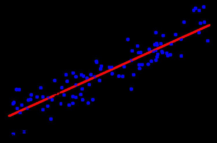
Regression analysis

In regression analysis, the following topics relate to goodness of fit:

Coefficient of determination (The R-squared measure of goodness of fit);

Lack-of-fit sum of squares;

Reduced chi-squared.

Categorical data

The following are examples that arise in the context of categorical data.

Pearson's chi-squared test

Pearson's chi-squared test uses a measure of goodness of fit which is the sum of differences between observed and expected outcome frequencies (that is, counts of observations), each squared and divided by the expectation:

χ 2 = ∑ i = 1 n ( O i − E i ) E i 2

where:

O_i = an observed frequency (i.e. count) for bin i E_i = an expected (theoretical) frequency for bin i, asserted by the null hypothesis.

The expected frequency is calculated by:

E i = ( F ( Y u ) − F ( Y l ) ) N

where:

F = the cumulative Distribution function for the distribution being tested. Y_u = the upper limit for class i, Y_l = the lower limit for class i, and N = the sample size

The resulting value can be compared to the chi-squared distribution to determine the goodness of fit. In order to determine the degrees of freedom of the chi-squared distribution, one takes the total number of observed frequencies and subtracts the number of estimated parameters. The test statistic follows, approximately, a chi-square distribution with (k − c) degrees of freedom where k is the number of non-empty cells and c is the number of estimated parameters (including location and scale parameters and shape parameters) for the distribution.

Example: equal frequencies of men and women

For example, to test the hypothesis that a random sample of 100 people has been drawn from a population in which men and women are equal in frequency, the observed number of men and women would be compared to the theoretical frequencies of 50 men and 50 women. If there were 44 men in the sample and 56 women, then

χ 2 = ( 44 − 50 ) 2 50 + ( 56 − 50 ) 2 50 = 1.44

If the null hypothesis is true (i.e., men and women are chosen with equal probability in the sample), the test statistic will be drawn from a chi-squared distribution with one degree of freedom. Though one might expect two degrees of freedom (one each for the men and women), we must take into account that the total number of men and women is constrained (100), and thus there is only one degree of freedom (2 − 1). Alternatively, if the male count is known the female count is determined, and vice versa.

Consultation of the chi-squared distribution for 1 degree of freedom shows that the probability of observing this difference (or a more extreme difference than this) if men and women are equally numerous in the population is approximately 0.23. This probability is higher than conventional criteria for statistical significance (.001-.05), so normally we would not reject the null hypothesis that the number of men in the population is the same as the number of women (i.e. we would consider our sample within the range of what we'd expect for a 50/50 male/female ratio.)

Binomial case

A binomial experiment is a sequence of independent trials in which the trials can result in one of two outcomes, success or failure. There are n trials each with probability of success, denoted by p. Provided that np_i ≫ 1 for every i (where i = 1, 2, ..., k), then

χ 2 = ∑ i = 1 k ( N i − n p i ) 2 n p i = ∑ a l l   c e l l s ( O − E ) 2 E .

This has approximately a chi-squared distribution with k − 1 degrees of freedom. The fact that there are k − 1 degrees of freedom is a consequence of the restriction ∑ N i = n . We know there are k observed cell counts, however, once any k − 1 are known, the remaining one is uniquely determined. Basically, one can say, there are only k − 1 freely determined cell counts, thus k − 1 degrees of freedom.

Other measures of fit

The likelihood ratio test statistic is a measure of the goodness of fit of a model, judged by whether an expanded form of the model provides a substantially improved fit.