Compressed sensing

Overview

A common goal of the engineering field of signal processing is to reconstruct a signal from a series of sampling measurements. In general, this task is impossible because there is no way to reconstruct a signal during the times that the signal is not measured. Nevertheless, with prior knowledge or assumptions about the signal, it turns out to be possible to perfectly reconstruct a signal from a series of measurements. Over time, engineers have improved their understanding of which assumptions are practical and how they can be generalized.

An early breakthrough in signal processing was the Nyquist–Shannon sampling theorem. It states that if the signal's highest frequency is less than half of the sampling rate, then the signal can be reconstructed perfectly. The main idea is that with prior knowledge about constraints on the signal’s frequencies, fewer samples are needed to reconstruct the signal.

Around 2004, Emmanuel Candès, Terence Tao, and David Donoho proved that given knowledge about a signal's sparsity, the signal may be reconstructed with even fewer samples than the sampling theorem requires. This idea is the basis of compressed sensing.

History

Compressed sensing relies on L1 techniques, which several other scientific fields have used historically. In statistics, the least squares method was complemented by the L 1 -norm, which was introduced by Laplace. Following the introduction of linear programming and Dantzig's simplex algorithm, the L 1 -norm was used in computational statistics. In statistical theory, the L 1 -norm was used by George W. Brown and later writers on median-unbiased estimators. It was used by Peter J. Huber and others working on robust statistics. The L 1 -norm was also used in signal processing, for example, in the 1970s, when seismologists constructed images of reflective layers within the earth based on data that did not seem to satisfy the Nyquist–Shannon criterion. It was used in matching pursuit in 1993, the LASSO estimator by Robert Tibshirani in 1996 and basis pursuit in 1998. There were theoretical results describing when these algorithms recovered sparse solutions, but the required type and number of measurements were sub-optimal and subsequently greatly improved by compressed sensing.

At first glance, compressed sensing might seem to violate the sampling theorem, because compressed sensing depends on the sparsity of the signal in question and not its highest frequency. This is a misconception, because the sampling theorem guarantees perfect reconstruction given sufficient, not necessary, conditions. A sampling method fundamentally different from classical fixed-rate sampling cannot "violate" the sampling theorem. Sparse signals with high frequency components can be highly under-sampled using compressed sensing compared to classical fixed-rate sampling.

Underdetermined linear system

An underdetermined system of linear equations has more unknowns than equations and generally has an infinite number of solutions. In order to choose a solution to such a system, one must impose extra constraints or conditions (such as smoothness) as appropriate.

In compressed sensing, one adds the constraint of sparsity, allowing only solutions which have a small number of nonzero coefficients. Not all underdetermined systems of linear equations have a sparse solution. However, if there is a unique sparse solution to the underdetermined system, then the compressed sensing framework allows the recovery of that solution.

Solution / reconstruction method

Compressed sensing takes advantage of the redundancy in many interesting signals—they are not pure noise. In particular, many signals are sparse, that is, they contain many coefficients close to or equal to zero, when represented in some domain. This is the same insight used in many forms of lossy compression.

Compressed sensing typically starts with taking a weighted linear combination of samples also called compressive measurements in a basis different from the basis in which the signal is known to be sparse. The results found by Emmanuel Candès, Justin Romberg, Terence Tao and David Donoho, showed that the number of these compressive measurements can be small and still contain nearly all the useful information. Therefore, the task of converting the image back into the intended domain involves solving an underdetermined matrix equation since the number of compressive measurements taken is smaller than the number of pixels in the full image. However, adding the constraint that the initial signal is sparse enables one to solve this underdetermined system of linear equations.

The least-squares solution to such problems is to minimize the L 2 norm—that is, minimize the amount of energy in the system. This is usually simple mathematically (involving only a matrix multiplication by the pseudo-inverse of the basis sampled in). However, this leads to poor results for many practical applications, for which the unknown coefficients have nonzero energy.

To enforce the sparsity constraint when solving for the underdetermined system of linear equations, one can minimize the number of nonzero components of the solution. The function counting the number of non-zero components of a vector was called the L 0 "norm" by David Donoho.

Candès. et al., proved that for many problems it is probable that the L 1 norm is equivalent to the L 0 norm, in a technical sense: This equivalence result allows one to solve the L 1 problem, which is easier than the L 0 problem. Finding the candidate with the smallest L 1 norm can be expressed relatively easily as a linear program, for which efficient solution methods already exist. When measurements may contain a finite amount of noise, basis pursuit denoising is preferred over linear programming, since it preserves sparsity in the face of noise and can be solved faster than an exact linear program.

Motivation and Applications

Role of TV regularization

Total variation can be seen as a non-negative real-valued functional defined on the space of real-valued functions (for the case of functions of one variable) or on the space of integrable functions (for the case of functions of several variables). For signals, especially, total variation refers to the integral of the absolute gradient of the signal. In signal and image reconstruction, it is applied as total variation regularization where the underlying principle is that signals with excessive details have high total variation and that removing these details, while retaining important information such as edges, would reduce the total variation of the signal and make the signal subject closer to the original signal in the problem.

For the purpose of signal and image reconstruction, l 1 minimization models are used. Other approaches also include the least-squares as has been discussed before in this article. These methods are extremely slow and return a not-so-perfect reconstruction of the signal. The current CS Regularization models attempt to address this problem by incorporating sparsity priors of the original image, one of which is the total variation (TV). Conventional TV approaches are designed to give piece-wise constant solutions. Some of these include (as discussed ahead) - constrained l1-minimization which uses an iterative scheme. This method, though fast, subsequently leads to over-smoothing of edges resulting in blurred image edges. TV methods with iterative re-weighting have been implemented to reduce the influence of large gradient value magnitudes in the images. This has been used in computed tomography (CT) reconstruction as a method known as edge-preserving total variation. However, as gradient magnitudes are used for estimation of relative penalty weights between the data fidelity and regularization terms, this method is not robust to noise and artifacts and accurate enough for CS image/signal reconstruction and, therefore, fails to preserve smaller structures.

Recent progress on this problem involves using an iteratively directional TV refinement for CS reconstruction. This method would have 2 stages: the first stage would estimate and refine the initial orientation field - which is defined as a noisy point-wise initial estimate, through edge-detection, of the given image. In the second stage, the CS reconstruction model is presented by utilizing directional TV regularizer. More details about these TV-based approaches - iteratively reweighted l1 minimization, edge-preserving TV and iterative model using directional orientation field and TV- are provided below.

Existing approaches

Iteratively reweighted l 1 minimization

In the CS reconstruction models using constrained l 1 minimization, larger coefficients are penalized heavily in the l 1 norm. It was proposed to have a weighted formulation of l 1 minimization designed to more democratically penalize nonzero coefficients. An iterative algorithm is used for constructing the appropriate weights. Each iteration requires solving one l 1 minimization problem by finding the local minimum of a concave penalty function that more closely resembles the l 0 norm. An additional parameter, usually to avoid any sharp transitions in the penalty function curve, is introduced into the iterative equation to ensure stability and so that a zero estimate in one iteration does not necessarily lead to a zero estimate in the next iteration. The method essentially involves using the current solution for computing the weights to be used in the next iteration.

Advantages and disadvantages

Early iterations may find inaccurate sample estimates, however this method will down-sample these at a later stage to give more weight to the smaller non-zero signal estimates. One of the disadvantages is the need for defining a valid starting point as a global minimum might not be obtained every time due to the concavity of the function. Another disadvantage is that this method tends to uniformly penalize the image gradient irrespective of the underlying image structures. This causes over-smoothing of edges, especially those of low contrast regions,subsequently leading to loss of low contrast information.The advantages of this method include: reduction of the sampling rate for sparse signals; reconstruction of the image while being robust to the removal of noise and other artifacts; and use of very few iterations. This can also help in recovering images with sparse gradients.

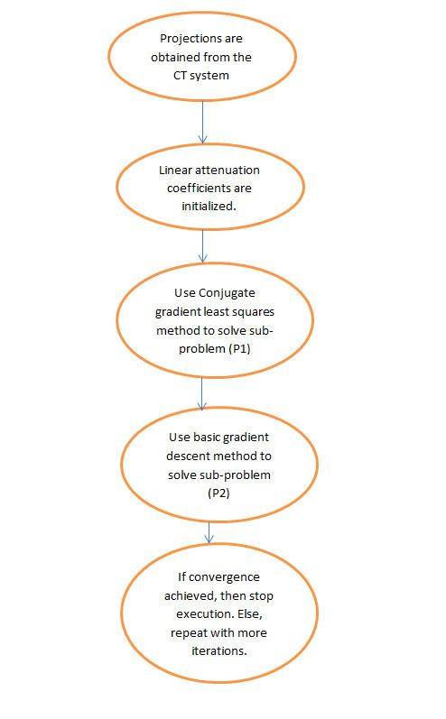
In the figure shown below, P1 refers to the first-step of the iterative reconstruction process, of the projection matrix P of the fan-beam geometry, which is constrained by the data fidelity term. This may contain noise and artifacts as no regularization is performed. The minimization of P1 is solved through the conjugate gradient least squares method. P2 refers to the second step of the iterative reconstruction process wherein it utilizes the edge-preserving total variation regularization term to remove noise and artifacts, and thus improve the quality of the reconstructed image/signal. The minimization of P2 is done through a simple gradient descent method. Convergence is determined by testing, after each iteration, for image positivity, by checking if f k − 1 = 0 for the case when f k − 1 < 0 (Note that f refers to the different x-ray linear attenuation coefficients at different voxels of the patient image).

Edge-preserving total variation (TV) based compressed sensing

This is an iterative CT reconstruction algorithm with edge-preserving TV regularization to reconstruct CT images from highly undersampled data obtained at low dose CT through low current levels (milliampere). In order to reduce the imaging dose, one of the approaches used is to reduce the number of x-ray projections acquired by the scanner detectors. However, this insufficient projection data which is used to reconstruct the CT image can cause streaking artifacts. Furthermore, using these insufficient projections in standard TV algorithms end up making the problem under-determined and thus leading to infinitely many possible solutions. In this method, an additional penalty weighted function is assigned to the original TV norm. This allows for easier detection of sharp discontinuities in intensity in the images and thereby adapt the weight to store the recovered edge information during the process of signal/image reconstruction. The parameter σ controls the amount of smoothing applied to the pixels at the edges to differentiate them from the non-edge pixels. The value of σ is changed adaptively based on the values of the histogram of the gradient magnitude so that a certain percentage of pixels have gradient values larger than σ . The edge-preserving total variation term, thus, becomes sparser and this speeds up the implementation. A two-step iteration process known as forward-backward splitting algorithm is used. The optimization problem is split into two sub-problems which are then solved with the conjugate gradient least squares method and the simple gradient descent method respectively. The method is stopped when the desired convergence has been achieved or if the maximum number of iterations is reached.

Advantages and disadvantages

Some of the disadvantages of this method are the absence of smaller structures in the reconstructed image and degradation of image resolution. This edge preserving TV algorithm, however, requires fewer iterations than the conventional TV algorithm. Analyzing the horizontal and vertical intensity profiles of the reconstructed images, it can be seen that there are sharp jumps at edge points and negligible, minor fluctuation at non-edge points. Thus, this method leads to low relative error and higher correlation as compared to the TV method. It also effectively suppresses and removes any form of image noise and image artifacts such as streaking.

Iterative model using a directional orientation field and directional total variation

To prevent over-smoothing of edges and texture details and to obtain a reconstructed CS image which is accurate and robust to noise and artifacts, this method is used. First, an initial estimate of the noisy point-wise orientation field of the image I , d ^ , is obtained. This noisy orientation field is defined so that it can be refined at a later stage to reduce the noise influences in orientation field estimation.A coarse orientation field estimation is then introduced based on structure tensor which is formulated as: J ρ ( ∇ I σ ) = G ρ ∗ ( ∇ I σ ⊗ ∇ I σ ) = ( J 11 J 12 J 12 J 22 ) . Here, J ρ refers to the structure tensor related with the image pixel point (i,j) having standard deviation ρ . G refers to the Gaussian kernel ( 0 , ρ 2 ) with standard deviation ρ . σ refers to the manually defined parameter for the image I below which the edge detection is insensitive to noise. ∇ I σ refers to the gradient of the image I and ( ∇ I σ ⊗ ∇ I σ ) refers to the tensor product obtained by using this gradient.

The structure tensor obtained is convolved with a Gaussian kernel G to improve the accuracy of the orientation estimate with σ being set to high values to account for the unknown noise levels. For every pixel (i,j) in the image, the structure tensor J is a symmetric and positive semi-definite matrix. Convolving all the pixels in the image with G , gives orthonormal eigen vectors ω and υ of the J matrix. ω points in the direction of the dominant orientation having the largest contrast and υ points in the direction of the structure orientation having the smallest contrast. The orientation field coarse initial estimation d ^ is defined as d ^ = υ. This estimate is accurate at strong edges. However, at weak edges or on regions with noise, its reliability decreases.

To overcome this drawback, a refined orientation model is defined in which the data term reduces the effect of noise and improves accuracy while the second penalty term with the L2-norm is a fidelity term which ensures accuracy of initial coarse estimation.

This orientation field is introduced into the directional total variation optimization model for CS reconstruction through the equation: m i n X ∥ ∇ X ∙ d ∥ 1 + λ 2   ∥ Y − Φ X ∥ 2 2 . X is the objective signal which needs to be recovered. Y is the corresponding measurement vector, d is the iterative refined orientation field and Φ is the CS measurement matrix. This method undergoes a few iterations ultimately leading to convergence. d ^ is the orientation field approximate estimation of the reconstructed image X k − 1 from the previous iteration (in order to check for convergence and the subsequent optical performance, the previous iteration is used). For the two vector fields represented by X and d , X ∙ d refers to the multiplication of respective horizontal and vertical vector elements of X and d followed by their subsequent addition. These equations are reduced to a series of convex minimization problems which are then solved with a combination of variable splitting and augmented Lagrangian (FFT-based fast solver with a closed form solution) methods. It (Augmented Lagrangian) is considered equivalent to the split Bregman iteration which ensures convergence of this method. The orientation field, d is defined as being equal to ( d h , d v ) , where d h , d v define the horizontal and vertical estimates of d .

The Augmented Lagrangian method for the orientation field, m i n X ∥ ∇ X ∙ d ∥ 1 + λ 2   ∥ Y − Φ X ∥ 2 2 , involves initializing d h , d v , H , V and then finding the approximate minimizer of L 1 with respect to these variables. The Lagrangian multipliers are then updated and the iterative process is stopped when convergence is achieved. For the iterative directional total variation refinement model, the augmented lagrangian method involves initializing X , P , Q , λ P , λ Q .

Here, H , V , P , Q are newly introduced variables where H = ∇ d h , V = ∇ d v , P = ∇ X , and Q = P ∙ d . λ H , λ V , λ P , λ Q are the Lagrangian multipliers for H , V , P , Q . For each iteration, the approximate minimizer of L 2 with respect to variables ( X , P , Q ) is calculated. And as in the field refinement model, the lagrangian multipliers are updated and the iterative process is stopped when convergence is achieved.

For the orientation field refinement model, the Lagrangian multipliers are updated in the iterative process as follows:

( λ H ) k = ( λ H ) k − 1 + γ H ( H k − ∇ ( d h ) k )

( λ V ) k = ( λ V ) k − 1 + γ V ( V k − ∇ ( d v ) k )

For the iterative directional total variation refinement model, the Lagrangian multipliers are updated as follows:

( λ P ) k = ( λ P ) k − 1 + γ P ( P k − ∇ ( X ) k )

( λ Q ) k = ( λ Q ) k − 1 + γ Q ( Q k − P k ∙ d )

Here, γ H , γ V , γ P , γ Q are positive constants.

Advantages and disadvantages

Based on Peak Signal-to-Noise Ratio (PSNR) and Structural Similarity Index (SSIM) metrics and known ground-truth images for testing performance, it is concluded that iterative directional total variation has a better reconstructed performance than the non-iterative methods in preserving edge and texture areas. The orientation field refinement model plays a major role in this improvement in performance as it increases the number of directionless pixels in the flat area while enhancing the orientation field consistency in the regions with edges.

Applications

The field of compressive sensing is related to several topics in signal processing and computational mathematics, such as underdetermined linear-systems, group testing, heavy hitters, sparse coding, multiplexing, sparse sampling, and finite rate of innovation. Its broad scope and generality has enabled several innovative CS-enhanced approaches in signal processing and compression, solution of inverse problems, design of radiating systems, radar and through-the-wall imaging, and antenna characterization. Imaging techniques having a strong affinity with compressive sensing include coded aperture and computational photography. Implementations of compressive sensing in hardware at different technology readiness levels is available.

Conventional CS reconstruction uses sparse signals (usually sampled at a rate less than the Nyquist sampling rate) for reconstruction through constrained l 1 minimization. One of the earliest applications of such an approach was in reflection seismology which used sparse reflected signals from band-limited data for tracking changes between sub-surface layers. When the LASSO model came into prominence in the 1990s as a statistical method for selection of sparse models, this method was further used in computational harmonic analysis for sparse signal representation from over-complete dictionaries. Some of the other applications include incoherent sampling of radar pulses. The work by Boyd et al. has applied the LASSO model- for selection of sparse models- towards analog to digital converters (the current ones use a sampling rate higher than the Nyquist rate along with the quantized Shannon representation). This would involve a parallel architecture in which the polarity of the analog signal changes at a high rate followed by digitizing the integral at the end of each time-interval to obtain the converted digital signal.

Photography

Compressed sensing is used in a mobile phone camera sensor. The approach allows a reduction in image acquisition energy per image by as much as a factor of 15 at the cost of complex decompression algorithms; the computation may require an off-device implementation.

Compressed sensing is used in single-pixel cameras from Rice University. Bell Labs employed the technique in a lensless single-pixel camera that takes stills using repeated snapshots of randomly chosen apertures from a grid. Image quality improves with the number of snapshots, and generally requires a small fraction of the data of conventional imaging, while eliminating lens/focus-related aberrations.

Holography

Compressed sensing can be used to improve image reconstruction in holography by increasing the number of voxels one can infer from a single hologram. It is also used for image retrieval from undersampled measurements in optical and millimeter-wave holography.

Facial recognition

Compressed sensing is being used in facial recognition applications.

Magnetic resonance imaging

Compressed sensing has been used to shorten magnetic resonance imaging scanning sessions on conventional hardware. Reconstruction methods include

Compressed sensing addresses the issue of high scan time by enabling faster acquisition by measuring fewer Fourier coefficients. This produces a high-quality image with relatively lower scan time. Another application (also discussed ahead) is for CT reconstruction with fewer X-ray projections. Compressed sensing, in this case, removes the high spatial gradient parts - mainly, image noise and artifacts. This holds tremendous potential as one can obtain high-resolution CT images at low radiation doses (through lower current-mA settings).

Network tomography

Compressed sensing has showed outstanding results in the application of network tomography to network management. Network delay estimation and network congestion detection can both be modeled as underdetermined systems of linear equations where the coefficient matrix is the network routing matrix. Moreover, in the Internet, network routing matrices usually satisfy the criterion for using compressed sensing.

Shortwave-infrared cameras

Commercial shortwave-infrared cameras based upon compressed sensing are available. These cameras have light sensitivity from 0.9 µm to 1.7 µm, which are wavelengths invisible to the human eye.

Aperture synthesis in radio astronomy

In the field of radio astronomy, compressed sensing has been proposed for deconvolving an interferometric image. In fact, the Högbom CLEAN algorithm that has been in use for the deconvolution of radio images since 1974, is similar to compressed sensing's matching pursuit algorithm.

Transmission electron microscopy

Compressed sensing combined with a moving aperture has been used to increase the acquisition rate of images in a transmission electron microscope. In scanning mode, compressive sensing combined with random scanning of the electron beam has enabled both faster acquisition and less electron dose, which allows for imaging of electron beam sensitive materials.