In statistics, the Huber loss is a loss function used in robust regression, that is less sensitive to outliers in data than the squared error loss. A variant for classification is also sometimes used.
The Huber loss function describes the penalty incurred by an estimation procedure f. Huber (1964) defines the loss function piecewise by
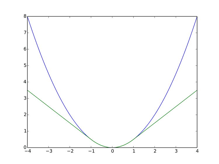
L δ ( a ) = { 1 2 a 2 for | a | ≤ δ , δ ( | a | − 1 2 δ ) , otherwise. This function is quadratic for small values of a, and linear for large values, with equal values and slopes of the different sections at the two points where | a | = δ . The variable a often refers to the residuals, that is to the difference between the observed and predicted values a = y − f ( x ) , so the former can be expanded to
L δ ( y , f ( x ) ) = { 1 2 ( y − f ( x ) ) 2 for | y − f ( x ) | ≤ δ , δ | y − f ( x ) | − 1 2 δ 2 otherwise. Two very commonly used loss functions are the squared loss, L ( a ) = a 2 , and the absolute loss, L ( a ) = | a | . The squared loss function results in an arithmetic mean-unbiased estimator, and the absolute-value loss function results in a median-unbiased estimator (in the one-dimensional case, and a geometric median-unbiased estimator for the multi-dimensional case). The squared loss has the disadvantage that it has the tendency to be dominated by outliers—when summing over a set of a 's (as in ∑ i = 1 n L ( a i ) ), the sample mean is influenced too much by a few particularly large a-values when the distribution is heavy tailed: in terms of estimation theory, the asymptotic relative efficiency of the mean is poor for heavy-tailed distributions.
As defined above, the Huber loss function is convex in a uniform neighborhood of its minimum a = 0 , at the boundary of this uniform neighborhood, the Huber loss function has a differentiable extension to an affine function at points a = − δ and a = δ . These properties allow it to combine much of the sensitivity of the mean-unbiased, minimum-variance estimator of the mean (using the quadratic loss function) and the robustness of the median-unbiased estimator (using the absolute value function).
The Pseudo-Huber loss function can be used as a smooth approximation of the Huber loss function, and ensures that derivatives are continuous for all degrees. It is defined as
L δ ( a ) = δ 2 ( 1 + ( a / δ ) 2 − 1 ) . As such, this function approximates a 2 / 2 for small values of a , and approximates a straight line with slope δ for large values of a .
While the above is the most common form, other smooth approximations of the Huber loss function also exist.
For classification purposes, a variant of the Huber loss called modified Huber is sometimes used. Given a prediction f ( x ) (a real-valued classifier score) and a true binary class label y ∈ { + 1 , − 1 } , the modified Huber loss is defined as
L ( y , f ( x ) ) = { max ( 0 , 1 − y f ( x ) ) 2 for y f ( x ) ≥ − 1 , − 4 y f ( x ) otherwise. The term max ( 0 , 1 − y f ( x ) ) is the hinge loss used by support vector machines; the quadratically smoothed hinge loss is a generalization of L .
The Huber loss function is used in robust statistics, M-estimation and additive modelling.