
 | ||
Purpose To roughly assess the probability distribution of a given variable by depicting the frequencies of observations occurring in certain ranges of values. | ||
A histogram is a graphical representation of the distribution of numerical data. It is an estimate of the probability distribution of a continuous variable (quantitative variable) and was first introduced by Karl Pearson. To construct a histogram, the first step is to "bin" the range of values—that is, divide the entire range of values into a series of intervals—and then count how many values fall into each interval. The bins are usually specified as consecutive, non-overlapping intervals of a variable. The bins (intervals) must be adjacent, and are often (but are not required to be) of equal size.
Contents
If the bins are of equal size, a rectangle is erected over the bin with height proportional to the frequency — the number of cases in each bin. A histogram may also be normalized to display "relative" frequencies. It then shows the proportion of cases that fall into each of several categories, with the sum of the heights equaling 1.
However, bins need not be of equal width; in that case, the erected rectangle is defined to have its area proportional to the frequency of cases in the bin. The vertical axis is then not the frequency but frequency density — the number of cases per unit of the variable on the horizontal axis. Examples of variable bin width are displayed on Census bureau data below.
As the adjacent bins leave no gaps, the rectangles of a histogram touch each other to indicate that the original variable is continuous.
Histograms give a rough sense of the density of the underlying distribution of the data, and often for density estimation: estimating the probability density function of the underlying variable. The total area of a histogram used for probability density is always normalized to 1. If the length of the intervals on the x-axis are all 1, then a histogram is identical to a relative frequency plot.
A histogram can be thought of as a simplistic kernel density estimation, which uses a kernel to smooth frequencies over the bins. This yields a smoother probability density function, which will in general more accurately reflect distribution of the underlying variable. The density estimate could be plotted as an alternative to the histogram, and is usually drawn as a curve rather than a set of boxes.
Another alternative is the average shifted histogram, which is fast to compute and gives a smooth curve estimate of the density without using kernels.
The histogram is one of the seven basic tools of quality control.
Histograms are sometimes confused with bar charts. A histogram is used for continuous data, where the bins represent ranges of data, while a bar chart is a plot of categorical variables. Some authors recommend that bar charts have gaps between the rectangles to clarify the distinction.
Etymology
The etymology of the word histogram is uncertain. Sometimes it is said to be derived from the Ancient Greek ἱστός (histos) – "anything set upright" (as the masts of a ship, the bar of a loom, or the vertical bars of a histogram); and γράμμα (gramma) – "drawing, record, writing". It is also said that Karl Pearson, who introduced the term in 1891, derived the name from "historical diagram".
Examples
This is a toy example:
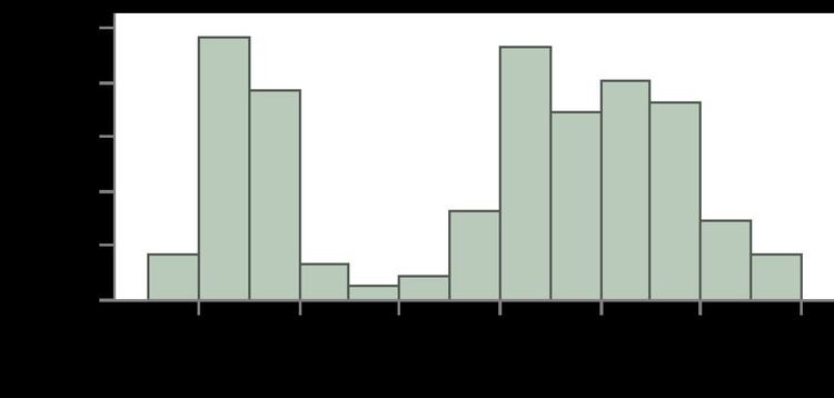
The words used to describe the patterns in a histogram are: "symmetric", "skewed left" or "right", "unimodal", "bimodal" or "multimodal".
It is a good idea to plot the data using several different bin widths to learn more about it. Here is an example on tips given in a restaurant.
Here are a couple more examples:
The U.S. Census Bureau found that there were 124 million people who work outside of their homes. Using their data on the time occupied by travel to work, the table below shows the absolute number of people who responded with travel times "at least 30 but less than 35 minutes" is higher than the numbers for the categories above and below it. This is likely due to people rounding their reported journey time. The problem of reporting values as somewhat arbitrarily rounded numbers is a common phenomenon when collecting data from people.
This histogram shows the number of cases per unit interval as the height of each block, so that the area of each block is equal to the number of people in the survey who fall into its category. The area under the curve represents the total number of cases (124 million). This type of histogram shows absolute numbers, with Q in thousands.
This histogram differs from the first only in the vertical scale. The area of each block is the fraction of the total that each category represents, and the total area of all the bars is equal to 1 (the fraction meaning "all"). The curve displayed is a simple density estimate. This version shows proportions, and is also known as a unit area histogram.
In other words, a histogram represents a frequency distribution by means of rectangles whose widths represent class intervals and whose areas are proportional to the corresponding frequencies: the height of each is the average frequency density for the interval. The intervals are placed together in order to show that the data represented by the histogram, while exclusive, is also contiguous. (E.g., in a histogram it is possible to have two connecting intervals of 10.5–20.5 and 20.5–33.5, but not two connecting intervals of 10.5–20.5 and 22.5–32.5. Empty intervals are represented as empty and not skipped.)
Mathematical definition
In a more general mathematical sense, a histogram is a function mi that counts the number of observations that fall into each of the disjoint categories (known as bins), whereas the graph of a histogram is merely one way to represent a histogram. Thus, if we let n be the total number of observations and k be the total number of bins, the histogram mi meets the following conditions:
Cumulative histogram
A cumulative histogram is a mapping that counts the cumulative number of observations in all of the bins up to the specified bin. That is, the cumulative histogram Mi of a histogram mj is defined as:
Number of bins and width
There is no "best" number of bins, and different bin sizes can reveal different features of the data. Grouping data is at least as old as Graunt's work in the 17th century, but no systematic guidelines were given until Sturges's work in 1926.
Using wider bins where the density is low reduces noise due to sampling randomness; using narrower bins where the density is high (so the signal drowns the noise) gives greater precision to the density estimation. Thus varying the bin-width within a histogram can be beneficial. Nonetheless, equal-width bins are widely used.
Some theoreticians have attempted to determine an optimal number of bins, but these methods generally make strong assumptions about the shape of the distribution. Depending on the actual data distribution and the goals of the analysis, different bin widths may be appropriate, so experimentation is usually needed to determine an appropriate width. There are, however, various useful guidelines and rules of thumb.
The number of bins k can be assigned directly or can be calculated from a suggested bin width h as:
The braces indicate the ceiling function.
which takes the square root of the number of data points in the sample (used by Excel histograms and many others).
Sturges' formula is derived from a binomial distribution and implicitly assumes an approximately normal distribution.
It implicitly bases the bin sizes on the range of the data and can perform poorly if n < 30, because the number of bins will be small—less than seven—and unlikely to show trends in the data well. It may also perform poorly if the data are not normally distributed.
The Rice Rule is presented as a simple alternative to Sturges's rule.
Doane's formula is a modification of Sturges' formula which attempts to improve its performance with non-normal data.
where
where
This approach of minimizing integrated mean squared error can be generalized beyond Normal distributions:
Here,
The Freedman–Diaconis rule is:
which is based on the interquartile range, denoted by IQR. It replaces 3.5σ of Scott's rule with 2 IQR, which is less sensitive than the standard deviation to outliers in data.
where
A good reason why the number of bins should be inversely proportional to
This simple cubic root choice can also be applied to bins with non-constant width.