Kernel density estimation

Definition

Let (x₁, x₂, …, x_n) be an independent and identically distributed sample drawn from some distribution with an unknown density ƒ. We are interested in estimating the shape of this function ƒ. Its kernel density estimator is

where K(•) is the kernel — a non-negative function that integrates to one and has mean zero — and h > 0 is a smoothing parameter called the bandwidth. A kernel with subscript h is called the scaled kernel and defined as K_h(x) = 1/h K(x/h). Intuitively one wants to choose h as small as the data allow; however, there is always a trade-off between the bias of the estimator and its variance. The choice of bandwidth is discussed in more detail below.

A range of kernel functions are commonly used: uniform, triangular, biweight, triweight, Epanechnikov, normal, and others. The Epanechnikov kernel is optimal in a mean square error sense, though the loss of efficiency is small for the kernels listed previously, and due to its convenient mathematical properties, the normal kernel is often used, which means K(x) = ϕ(x), where ϕ is the standard normal density function.

The construction of a kernel density estimate finds interpretations in fields outside of density estimation. For example, in thermodynamics, this is equivalent to the amount of heat generated when heat kernels (the fundamental solution to the heat equation) are placed at each data point locations x_i. Similar methods are used to construct discrete Laplace operators on point clouds for manifold learning.

Kernel density estimates are closely related to histograms, but can be endowed with properties such as smoothness or continuity by using a suitable kernel. To see this, we compare the construction of histogram and kernel density estimators, using these 6 data points: x₁ = −2.1, x₂ = −1.3, x₃ = −0.4, x₄ = 1.9, x₅ = 5.1, x₆ = 6.2. For the histogram, first the horizontal axis is divided into sub-intervals or bins which cover the range of the data. In this case, we have 6 bins each of width 2. Whenever a data point falls inside this interval, we place a box of height 1/12. If more than one data point falls inside the same bin, we stack the boxes on top of each other.

For the kernel density estimate, we place a normal kernel with variance 2.25 (indicated by the red dashed lines) on each of the data points x_i. The kernels are summed to make the kernel density estimate (solid blue curve). The smoothness of the kernel density estimate is evident compared to the discreteness of the histogram, as kernel density estimates converge faster to the true underlying density for continuous random variables.

Bandwidth selection

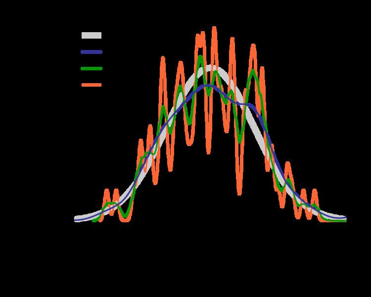
The bandwidth of the kernel is a free parameter which exhibits a strong influence on the resulting estimate. To illustrate its effect, we take a simulated random sample from the standard normal distribution (plotted at the blue spikes in the rug plot on the horizontal axis). The grey curve is the true density (a normal density with mean 0 and variance 1). In comparison, the red curve is undersmoothed since it contains too many spurious data artifacts arising from using a bandwidth h = 0.05, which is too small. The green curve is oversmoothed since using the bandwidth h = 2 obscures much of the underlying structure. The black curve with a bandwidth of h = 0.337 is considered to be optimally smoothed since its density estimate is close to the true density.

The most common optimality criterion used to select this parameter is the expected L₂ risk function, also termed the mean integrated squared error:

Under weak assumptions on ƒ and K, MISE (h) = AMISE(h) + o(1/(nh) + h⁴) where o is the little o notation. The AMISE is the Asymptotic MISE which consists of the two leading terms

where R ( g ) = ∫ g ( x ) 2 d x for a function g, m 2 ( K ) = ∫ x 2 K ( x ) d x and ƒ'' is the second derivative of ƒ. The minimum of this AMISE is the solution to this differential equation

or

Neither the AMISE nor the h_AMISE formulas are able to be used directly since they involve the unknown density function ƒ or its second derivative ƒ'', so a variety of automatic, data-based methods have been developed for selecting the bandwidth. Many review studies have been carried out to compare their efficacies, with the general consensus that the plug-in selectors and cross validation selectors are the most useful over a wide range of data sets.

Substituting any bandwidth h which has the same asymptotic order n^−1/5 as h_AMISE into the AMISE gives that AMISE(h) = O(n^−4/5), where O is the big o notation. It can be shown that, under weak assumptions, there cannot exist a non-parametric estimator that converges at a faster rate than the kernel estimator. Note that the n^−4/5 rate is slower than the typical n⁻¹ convergence rate of parametric methods.

If the bandwidth is not held fixed, but is varied depending upon the location of either the estimate (balloon estimator) or the samples (pointwise estimator), this produces a particularly powerful method termed adaptive or variable bandwidth kernel density estimation.

Bandwidth selection for kernel density estimation of heavy-tailed distributions is said to be relatively difficult.

A rule-of-thumb bandwidth estimator

If Gaussian basis functions are used to approximate univariate data, and the underlying density being estimated is Gaussian, the optimal choice for h (that is, the bandwidth that minimises the mean integrated squared error) is

where σ ^ is the standard deviation of the samples. This approximation is termed the normal distribution approximation, Gaussian approximation, or Silverman's (1986) rule of thumb. While this rule of thumb is easy to compute, it should be used with caution as it can yield widely inaccurate estimates when the density is not close to being normal. For example, consider estimating the bimodal Gaussian mixture:

from a sample of 200 points. The figure on the right below shows the true density and two kernel density estimates --- one using the rule-of-thumb bandwidth, and the other using a solve-the-equation bandwidth. The estimate based on the rule-of-thumb bandwidth is significantly oversmoothed. The Matlab script for this example uses kde.m and is given below.

Relation to the characteristic function density estimator

Given the sample (x₁, x₂, …, x_n), it is natural to estimate the characteristic function φ(t) = E[e^itX] as

Knowing the characteristic function, it is possible to find the corresponding probability density function through the Fourier transform formula. One difficulty with applying this inversion formula is that it leads to a diverging integral, since the estimate φ ^ ( t ) is unreliable for large t’s. To circumvent this problem, the estimator φ ^ ( t ) is multiplied by a damping function ψ_h(t) = ψ(ht), which is equal to 1 at the origin and then falls to 0 at infinity. The “bandwidth parameter” h controls how fast we try to dampen the function φ ^ ( t ) . In particular when h is small, then ψ_h(t) will be approximately one for a large range of t’s, which means that φ ^ ( t ) remains practically unaltered in the most important region of t’s.

The most common choice for function ψ is either the uniform function ψ(t) = 1{−1 ≤ t ≤ 1}, which effectively means truncating the interval of integration in the inversion formula to [−1/h, 1/h], or the gaussian function ψ(t) = e^−π t2. Once the function ψ has been chosen, the inversion formula may be applied, and the density estimator will be

where K is the Fourier transform of the damping function ψ. Thus the kernel density estimator coincides with the characteristic function density estimator.

Statistical implementation

A non-exhaustive list of software implementations of kernel density estimators includes: