
 | ||
In descriptive statistics, the interquartile range (IQR), also called the midspread or middle 50%, or technically H-spread, is a measure of statistical dispersion, being equal to the difference between 75th and 25th percentiles, or between upper and lower quartiles, IQR = Q3 − Q1. In other words, the IQR is the 1st quartile subtracted from the 3rd quartile; these quartiles can be clearly seen on a box plot on the data. It is a trimmed estimator, defined as the 25% trimmed range, and is the most significant basic robust measure of scale.
Contents
- Use
- Data set in a plain text box plot
- Interquartile range of distributions
- Interquartile range test for normality of distribution
- Interquartile range and outliers
- References
The interquartile range (IQR) is a measure of variability, based on dividing a data set into quartiles. Quartiles divide a rank-ordered data set into four equal parts. The values that separate parts are called the first, second, and third quartiles; and they are denoted by Q1, Q2, and Q3, respectively.
Use
Unlike total range, the interquartile range has a breakdown point of 25%, and is thus often preferred to the total range.
The IQR is used to build box plots, simple graphical representations of a probability distribution.
For a symmetric distribution (where the median equals the midhinge, the average of the first and third quartiles), half the IQR equals the median absolute deviation (MAD).
The median is the corresponding measure of central tendency.
The IQR can be used to identify outliers (see below).
The quartile deviation or semi-interquartile range is defined as half the IQR.
For the data in this table the interquartile range is IQR = Q3 − Q1 = 119 − 31 = 88.
Data set in a plain-text box plot
+-----+-+ o * |-------| | |---| +-----+-+ +---+---+---+---+---+---+---+---+---+---+---+---+ number line 0 1 2 3 4 5 6 7 8 9 10 11 12For the data set in this box plot:
Interquartile range of distributions
The interquartile range of a continuous distribution can be calculated by integrating the probability density function (which yields the cumulative distribution function — any other means of calculating the CDF will also work). The lower quartile, Q1, is a number such that integral of the PDF from -∞ to Q1 equals 0.25, while the upper quartile, Q3, is such a number that the integral from -∞ to Q3 equals 0.75; in terms of the CDF, the quartiles can be defined as follows:
where CDF−1 is the quantile function.
The interquartile range and median of some common distributions are shown below
Interquartile range test for normality of distribution
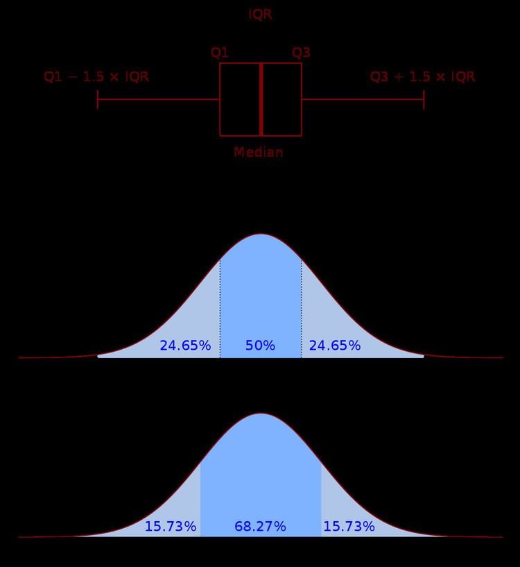
The IQR, mean, and standard deviation of a population P can be used in a simple test of whether or not P is normally distributed, or Gaussian. If P is normally distributed, then the standard score of the first quartile, z1, is -0.67, and the standard score of the third quartile, z3, is +0.67. Given mean = X and standard deviation = σ for P, if P is normally distributed, the first quartile
and the third quartile
If the actual values of the first or third quartiles differ substantially from the calculated values, P is not normally distributed. However, a normal distribution can be trivially perturbed to maintain its Q1 and Q2 std. scores at 0.67 and -0.67 and not be normally distributed (so the above test would produce a false positive). A better test of normality, such as Q-Q plot would be indicated here.
Interquartile range and outliers
The interquartile range is often used to find outliers in data. Outliers are observations that fall below Q1 − 1.5 IQR or above Q3 + 1.5 IQR. In a boxplot, the highest and lowest occurring value within this limit are drawn as bar of the whiskers, and the outliers as individual points.