Generalized beta distribution - Alchetron, the free social encyclopedia

In probability and statistics, the generalized beta distribution is a continuous probability distribution with five parameters, including more than thirty named distributions as limiting or special cases. It has been used in the modeling of income distribution, stock returns, as well as in regression analysis. The exponential generalized Beta (EGB) distribution follows directly from the GB and generalizes other common distributions.

Definition

A generalized beta random variable, Y, is defined by the following probability density function:

G B ( y ; a , b , c , p , q ) = | a | y a p − 1 ( 1 − ( 1 − c ) ( y / b ) a ) q − 1 b a p B ( p , q ) ( 1 + c ( y / b ) a ) p + q for 0 < y a < b a 1 − c ,

and zero otherwise. Here the parameters satisfy 0 ≤ c ≤ 1 and b , p , and q positive. The function B(p,q) is the beta function.

Moments

It can be shown that the hth moment can be expressed as follows:

E G B ⁡ ( Y h ) = b h B ( p + h / a , q ) B ( p , q ) 2 F 1 [ p + h / a , h / a ; c p + q + h / a ; ] ,

where 2 F 1 denotes the hypergeometric series (which converges for all h if c<1, or for all h/a<q if c=1 ).

The generalized beta encompasses a number of distributions in its family as special cases. Listed below are its three direct descendants, or sub-families.

Generalized beta of first kind (GB1)

The generalized beta of the first kind is defined by the following pdf:

G B 1 ( y ; a , b , p , q ) = | a | y a p − 1 ( 1 − ( y / b ) a ) q − 1 b a p B ( p , q )

for 0 < y a < b a where b , p , and q are positive. It is easily verified that

G B 1 ( y ; a , b , p , q ) = G B ( y ; a , b , c = 0 , p , q ) .

The moments of the GB1 are given by

E G B 1 ⁡ ( Y h ) = b h B ( p + h / a , q ) B ( p , q ) .

The GB1 includes the beta of the first kind (B1), generalized gamma(GG), and Pareto as special cases:

B 1 ( y ; b , p , q ) = G B 1 ( y ; a = 1 , b , p , q ) , G G ( y ; a , β , p ) = lim q → ∞ G B 1 ( y ; a , b = q 1 / a β , p , q ) , P A R E T O ( y ; b , p ) = G B 1 ( y ; a = − 1 , b , p , q = 1 ) .

Generalized beta of the second kind (GB2)

The GB2 (also known as the Generalized Beta Prime) is defined by the following pdf:

G B 2 ( y ; a , b , p , q ) = | a | y a p − 1 b a p B ( p , q ) ( 1 + ( y / b ) a ) p + q

for 0 < y < ∞ and zero otherwise. One can verify that

G B 2 ( y ; a , b , p , q ) = G B ( y ; a , b , c = 1 , p , q ) .

The moments of the GB2 are given by

E G B 2 ⁡ ( Y h ) = b h B ( p + h / a , q − h / a ) B ( p , q ) .

The GB2 nests common distributions such as the generalized gamma (GG), Burr type 3, Burr type 12, Dagum, lognormal, Weibull, gamma, Lomax, F statistic, Fisk or Rayleigh, chi-square, half-normal, half-Student's t, exponential, and the log-logistic.

Beta

The beta distribution (B) is defined by:

B ( y ; b , c , p , q ) = y p − 1 ( 1 − ( 1 − c ) ( y / b ) ) q − 1 b p B ( p , q ) ( 1 + c ( y / b ) ) p + q

for 0 < y < b / ( 1 − c ) and zero otherwise. Its relation to the GB is seen below:

B ( y ; b , c , p , q ) = G B ( y ; a = 1 , b , c , p , q ) .

The beta family includes the betas of the first and second kind (B1 and B2, where the B2 is also referred to as the Beta prime), which correspond to c = 0 and c = 1, respectively.

Generalized Gamma

The generalized gamma distribution (GG) is a limiting case of the GB2. The PDF is defined by:

G G ( y ; a , β , p ) = lim q → ∞ G B 2 ( y , a , b = q 1 / a β , p , q ) = | a | y a p − 1 e − ( y / β ) a β a Γ ( p )

with the h th moments given by

E ⁡ ( Y G G h ) = β h Γ ( p + h / a ) Γ ( p ) .

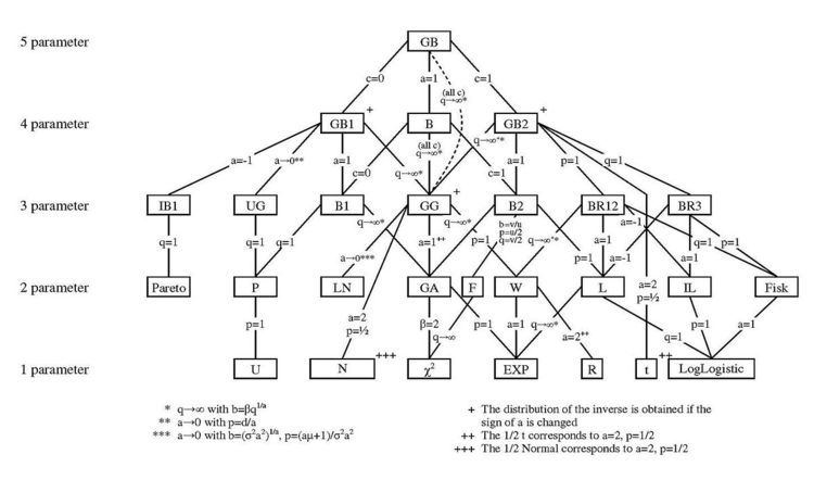
A figure showing the relationship between the GB and its special and limiting cases is included above (see McDonald and Xu (1995) ).

Exponential generalized beta distribution

Letting Y ∼ G B ( y ; a , b , c , p , q ) , the random variable Z = ln ⁡ ( Y ) , with re-parametrization, is distributed as an exponential generalized beta (EGB), with the following pdf:

E G B ( z ; δ , σ , c , p , q ) = e p ( z − δ ) / σ ( 1 − ( 1 − c ) e ( z − δ ) / σ ) q − 1 | σ | B ( p , q ) ( 1 + c e ( z − δ ) / σ ) p + q

for − ∞ < z − δ σ < ln ⁡ ( 1 1 − c ) , and zero otherwise. The EGB includes generalizations of the Gompertz, Gumbell, extreme value type I, logistic, Burr-2, exponential, and normal distributions.

Included is a figure showing the relationship between the EGB and its special and limiting cases.

Moment generating function

Using similar notation as above, the moment-generating function of the EGB can be expressed as follows:

M E G B ( Z ) = e δ t B ( p + t σ , q ) B ( p , q ) 2 F 1 [ p + t σ , t σ ; c p + q + t σ ; ] .

Applications

The flexibility provided by the GB family is used in modeling the distribution of:

distribution of income

hazard functions

stock returns

insurance losses

Applications involving members of the EGB family include:

partially adaptive estimation of regression

time series models

(G)ARCH models

Distribution of Income

The GB2 and several of its special and limiting cases have been widely used as models for the distribution of income. For some early examples see Thurow (1970), Dagum (1977), Singh and Maddala (1976), and McDonald (1984). Maximum likelihood estimations using individual, grouped, or top-coded data are easily performed with these distributions.

Measures of inequality, such as the Gini index (G), Pietra index (P), and Theil index (T) can be expressed in terms of the distributional parameters, as given by McDonald and Ransom (2008):

G = ( 1 2 μ ) E ⁡ ( | Y − X | ) = ( P 1 2 μ ) ∫ 0 ∞ ∫ 0 ∞ | x − y | f ( x ) f ( y ) d x d y = 1 − ∫ 0 ∞ ( 1 − F ( y ) ) 2 d y ∫ 0 ∞ ( 1 − F ( y ) ) d y P = ( 1 2 μ ) E ⁡ ( | Y − μ | ) = ( 1 2 μ ) ∫ 0 ∞ | y − μ | f ( y ) d y T = E ⁡ ( ln ⁡ ( Y / μ ) Y / μ ) = ∫ 0 ∞ ( y / μ ) ln ⁡ ( y / μ ) f ( y ) d y

Hazard Functions

The hazard function, h(s), where f(s) is a pdf and F(s) the corresponding cdf, is defined by

h ( s ) = f ( s ) 1 − F ( s )

Hazard functions are useful in many applications, such as modeling unemployment duration, the failure time of products or life expectancy. Taking a specific example, if s denotes the length of life, then h(s) is the rate of death at age s, given that an individual has lived up to age s. The shape of the hazard function for mortality data might appear as follows: The hazard function h(s) exhibits decreasing mortality in the first few months of life, then a period of relatively constant mortality and finally an increasing probability of death at older ages.

Special cases of the generalized beta distribution offer more flexibility in modeling the shape of the hazard function, which can call for "∪" or "∩" shapes or strictly increasing (denoted by I) or decreasing (denoted by D) lines. The generalized gamma is "∪"-shaped for a>1 and p<1/a, "∩"-shaped for a<1 and p>1/a, I-shaped for a>1 and p>1/a and D-shaped for a<1 and p>1/a. This is summarized in the figure below.

References

Generalized beta distribution Wikipedia

(Text) CC BY-SA

Contents