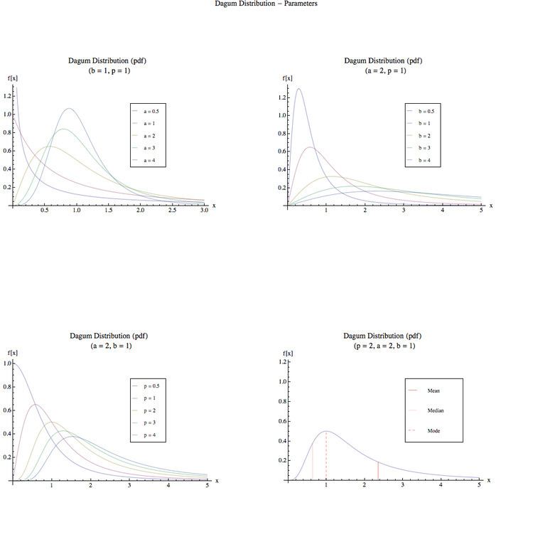
 | ||
Parameters Support x > 0 {\displaystyle x>0} PDF a p x ( ( x b ) a p ( ( x b ) a + 1 ) p + 1 ) {\displaystyle {\frac {ap}{x}}\left({\frac {({\tfrac {x}{b}})^{ap}}{\left(({\tfrac {x}{b}})^{a}+1\right)^{p+1}}}\right)} CDF ( 1 + ( x b ) − a ) − p {\displaystyle {\left(1+{\left({\frac {x}{b}}\right)}^{-a}\right)}^{-p}} Mean { − b a Γ ( − 1 a ) Γ ( 1 a + p ) Γ ( p ) if a > 1 Indeterminate otherwise {\displaystyle {\begin{cases}-{\frac {b}{a}}{\frac {\Gamma \left(-{\tfrac {1}{a}}\right)\Gamma \left({\tfrac {1}{a}}+p\right)}{\Gamma (p)}}&{\text{if}}\ a>1\\{\text{Indeterminate}}&{\text{otherwise}}\ \end{cases}}} Median b ( − 1 + 2 1 p ) − 1 a {\displaystyle b{\left(-1+2^{\tfrac {1}{p}}\right)}^{-{\tfrac {1}{a}}}} | ||
The Dagum distribution is a continuous probability distribution defined over positive real numbers. It is named after Camilo Dagum, who proposed it in a series of papers in the 1970s. The Dagum distribution arose from several variants of a new model on the size distribution of personal income and is mostly associated with the study of income distribution. There is both a three-parameter specification (Type I) and a four-parameter specification (Type II) of the Dagum distribution; a summary of the genesis of this distribution can be found in "A Guide to the Dagum Distributions". A general source on statistical size distributions often cited in work using the Dagum distribution is Statistical Size Distributions in Economics and Actuarial Sciences.
Contents
Definition
The cumulative distribution function of the Dagum distribution (Type I) is given by
The corresponding probability density function is given by
The quantile function is given by
The Dagum distribution can be derived as a special case of the Generalized Beta II (GB2) distribution (a generalization of the Beta prime distribution):
There is also an intimate relationship between the Dagum and Singh-Maddala distribution.
The cumulative distribution function of the Dagum (Type II) distribution adds a point mass at the origin and then follows a Dagum (Type I) distribution over the rest of the support (i.e. over the positive halfline)
Use in economics
The Dagum distribution if often used to model income and wealth distribution. The relation between the Dagum Type I and the gini coefficient is summarized in the formula below:
Note that this value is independent on the scale-parameter,
Although the Dagum distribution is not the only three parameter distribution used to model income distribution it is usually the most appropriate.
