
 | ||
Parameters c > 0 {\displaystyle c>0\!} k > 0 {\displaystyle k>0\!} Support x > 0 {\displaystyle x>0\!} PDF c k x c − 1 ( 1 + x c ) k + 1 {\displaystyle ck{\frac {x^{c-1}}{(1+x^{c})^{k+1}}}\!} CDF 1 − ( 1 + x c ) − k {\displaystyle 1-\left(1+x^{c}\right)^{-k}} Mean μ 1 = k B ( k − 1 / c , 1 + 1 / c ) {\displaystyle \mu _{1}=k\operatorname {\mathrm {B} } (k-1/c,\,1+1/c)} where Β() is the beta function Median ( 2 1 k − 1 ) 1 c {\displaystyle \left(2^{\frac {1}{k}}-1\right)^{\frac {1}{c}}} | ||
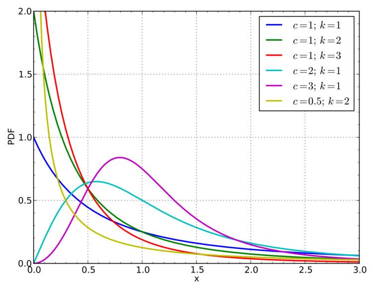
In probability theory, statistics and econometrics, the Burr Type XII distribution or simply the Burr distribution is a continuous probability distribution for a non-negative random variable. It is also known as the Singh–Maddala distribution and is one of a number of different distributions sometimes called the "generalized log-logistic distribution". It is most commonly used to model household income (See: Household income in the U.S. and compare to magenta graph at right).
The Burr (Type XII) distribution has probability density function:
and cumulative distribution function:
Note when c=1, the Burr distribution becomes the Pareto Type II (Lomax) distribution. When k=1, the Burr distribution is a special case of the Champernowne distribution, often referred to as the Fisk distribution.
The Burr Type XII distribution is a member of a system of continuous distributions introduced by Irving W. Burr (1942), which comprises 12 distributions.