Finite difference time domain method

Updated on Jan 10, 2024

Edit

Comment

Finite-difference time-domain or Yee's method (named after the Chinese American applied mathematician Kane S. Yee, born 1934) is a numerical analysis technique used for modeling computational electrodynamics (finding approximate solutions to the associated system of differential equations). Since it is a time-domain method, FDTD solutions can cover a wide frequency range with a single simulation run, and treat nonlinear material properties in a natural way.

The FDTD method belongs in the general class of grid-based differential numerical modeling methods (finite difference methods). The time-dependent Maxwell's equations (in partial differential form) are discretized using central-difference approximations to the space and time partial derivatives. The resulting finite-difference equations are solved in either software or hardware in a leapfrog manner: the electric field vector components in a volume of space are solved at a given instant in time; then the magnetic field vector components in the same spatial volume are solved at the next instant in time; and the process is repeated over and over again until the desired transient or steady-state electromagnetic field behavior is fully evolved.

History

Finite difference schemes for time-dependent PDEs have been employed for many years in computational fluid dynamics problems, including the idea of using centered finite difference operators on staggered grids in space and time to achieve second-order accuracy. The novelty of Kane Yee's FDTD scheme, presented in his seminal 1966 paper, was to apply centered finite difference operators on staggered grids in space and time for each electric and magnetic vector field component in Maxwell's curl equations. The descriptor "Finite-difference time-domain" and its corresponding "FDTD" acronym were originated by Allen Taflove in 1980. Since about 1990, FDTD techniques have emerged as primary means to computationally model many scientific and engineering problems dealing with electromagnetic wave interactions with material structures. Current FDTD modeling applications range from near-DC (ultralow-frequency geophysics involving the entire Earth-ionosphere waveguide) through microwaves (radar signature technology, antennas, wireless communications devices, digital interconnects, biomedical imaging/treatment) to visible light (photonic crystals, nanoplasmonics, solitons, and biophotonics). In 2006, an estimated 2,000 FDTD-related publications appeared in the science and engineering literature (see Popularity). As of 2013, there are at least 25 commercial/proprietary FDTD software vendors; 13 free-software/open-source-software FDTD projects; and 2 freeware/closed-source FDTD projects, some not for commercial use (see External links).

Development of FDTD and Maxwell's equations

An appreciation of the basis, technical development, and possible future of FDTD numerical techniques for Maxwell’s equations can be developed by first considering their history. The following lists some of the key publications in this area.

FDTD models and methods

When Maxwell's differential equations are examined, it can be seen that the change in the E-field in time (the time derivative) is dependent on the change in the H-field across space (the curl). This results in the basic FDTD time-stepping relation that, at any point in space, the updated value of the E-field in time is dependent on the stored value of the E-field and the numerical curl of the local distribution of the H-field in space.

The H-field is time-stepped in a similar manner. At any point in space, the updated value of the H-field in time is dependent on the stored value of the H-field and the numerical curl of the local distribution of the E-field in space. Iterating the E-field and H-field updates results in a marching-in-time process wherein sampled-data analogs of the continuous electromagnetic waves under consideration propagate in a numerical grid stored in the computer memory.

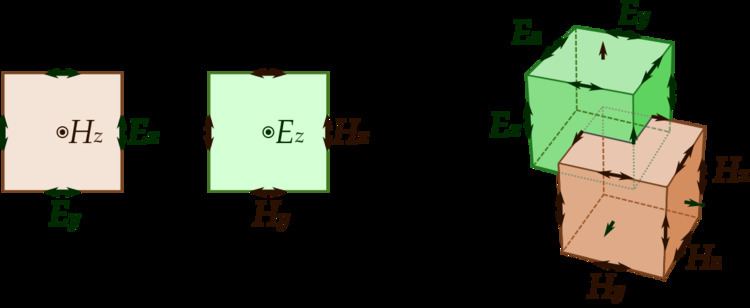
This description holds true for 1-D, 2-D, and 3-D FDTD techniques. When multiple dimensions are considered, calculating the numerical curl can become complicated. Kane Yee's seminal 1966 paper proposed spatially staggering the vector components of the E-field and H-field about rectangular unit cells of a Cartesian computational grid so that each E-field vector component is located midway between a pair of H-field vector components, and conversely. This scheme, now known as a Yee lattice, has proven to be very robust, and remains at the core of many current FDTD software constructs.

Furthermore, Yee proposed a leapfrog scheme for marching in time wherein the E-field and H-field updates are staggered so that E-field updates are conducted midway during each time-step between successive H-field updates, and conversely. On the plus side, this explicit time-stepping scheme avoids the need to solve simultaneous equations, and furthermore yields dissipation-free numerical wave propagation. On the minus side, this scheme mandates an upper bound on the time-step to ensure numerical stability. As a result, certain classes of simulations can require many thousands of time-steps for completion.

Using the FDTD method

To implement an FDTD solution of Maxwell's equations, a computational domain must first be established. The computational domain is simply the physical region over which the simulation will be performed. The E and H fields are determined at every point in space within that computational domain. The material of each cell within the computational domain must be specified. Typically, the material is either free-space (air), metal, or dielectric. Any material can be used as long as the permeability, permittivity, and conductivity are specified.

The permittivity of dispersive materials in tabular form cannot be directly substituted into the FDTD scheme. Instead, it can be approximated using multiple Debye, Drude, Lorentz or critical point terms. This approximation can be obtained using open fitting programs and does not necessarily have physical meaning.

Once the computational domain and the grid materials are established, a source is specified. The source can be current on a wire, applied electric field or impinging plane wave. In the last case FDTD can be used to simulate light scattering from arbitrary shaped objects, planar periodic structures at various incident angles, and photonic band structure of infinite periodic structures.

Since the E and H fields are determined directly, the output of the simulation is usually the E or H field at a point or a series of points within the computational domain. The simulation evolves the E and H fields forward in time.

Processing may be done on the E and H fields returned by the simulation. Data processing may also occur while the simulation is ongoing.

While the FDTD technique computes electromagnetic fields within a compact spatial region, scattered and/or radiated far fields can be obtained via near-to-far-field transformations.

Strengths of FDTD modeling

Every modeling technique has strengths and weaknesses, and the FDTD method is no different.

FDTD is a versatile modeling technique used to solve Maxwell's equations. It is intuitive, so users can easily understand how to use it and know what to expect from a given model.

FDTD is a time-domain technique, and when a broadband pulse (such as a Gaussian pulse) is used as the source, then the response of the system over a wide range of frequencies can be obtained with a single simulation. This is useful in applications where resonant frequencies are not exactly known, or anytime that a broadband result is desired.

Since FDTD calculates the E and H fields everywhere in the computational domain as they evolve in time, it lends itself to providing animated displays of the electromagnetic field movement through the model. This type of display is useful in understanding what is going on in the model, and to help ensure that the model is working correctly.

The FDTD technique allows the user to specify the material at all points within the computational domain. A wide variety of linear and nonlinear dielectric and magnetic materials can be naturally and easily modeled.

FDTD allows the effects of apertures to be determined directly. Shielding effects can be found, and the fields both inside and outside a structure can be found directly or indirectly.

FDTD uses the E and H fields directly. Since most EMI/EMC modeling applications are interested in the E and H fields, it is convenient that no conversions must be made after the simulation has run to get these values.

Weaknesses of FDTD modeling

Since FDTD requires that the entire computational domain be gridded, and the grid spatial discretization must be sufficiently fine to resolve both the smallest electromagnetic wavelength and the smallest geometrical feature in the model, very large computational domains can be developed, which results in very long solution times. Models with long, thin features, (like wires) are difficult to model in FDTD because of the excessively large computational domain required. Methods such as Eigenmode Expansion can offer a more efficient alternative as they do not require a fine grid along the z-direction.

There is no way to determine unique values for permittivity and permeability at a material interface.

Space and time steps must satisfy the CFL condition, or the leapfrog integration used to solve the partial differential equation is likely to become unstable.

FDTD finds the E/H fields directly everywhere in the computational domain. If the field values at some distance are desired, it is likely that this distance will force the computational domain to be excessively large. Far-field extensions are available for FDTD, but require some amount of postprocessing.

Since FDTD simulations calculate the E and H fields at all points within the computational domain, the computational domain must be finite to permit its residence in the computer memory. In many cases this is achieved by inserting artificial boundaries into the simulation space. Care must be taken to minimize errors introduced by such boundaries. There are a number of available highly effective absorbing boundary conditions (ABCs) to simulate an infinite unbounded computational domain. Most modern FDTD implementations instead use a special absorbing "material", called a perfectly matched layer (PML) to implement absorbing boundaries.

Because FDTD is solved by propagating the fields forward in the time domain, the electromagnetic time response of the medium must be modeled explicitly. For an arbitrary response, this involves a computationally expensive time convolution, although in most cases the time response of the medium (or Dispersion (optics)) can be adequately and simply modeled using either the recursive convolution (RC) technique, the auxiliary differential equation (ADE) technique, or the Z-transform technique. An alternative way of solving Maxwell's equations that can treat arbitrary dispersion easily is the Pseudospectral Spatial-Domain method (PSSD), which instead propagates the fields forward in space.

Grid truncation techniques

The most commonly used grid truncation techniques for open-region FDTD modeling problems are the Mur absorbing boundary condition (ABC), the Liao ABC, and various perfectly matched layer (PML) formulations. The Mur and Liao techniques are simpler than PML. However, PML (which is technically an absorbing region rather than a boundary condition per se) can provide orders-of-magnitude lower reflections. The PML concept was introduced by J.-P. Berenger in a seminal 1994 paper in the Journal of Computational Physics. Since 1994, Berenger's original split-field implementation has been modified and extended to the uniaxial PML (UPML), the convolutional PML (CPML), and the higher-order PML. The latter two PML formulations have increased ability to absorb evanescent waves, and therefore can in principle be placed closer to a simulated scattering or radiating structure than Berenger's original formulation.

To reduce undesired numerical reflection from the PML additional back absorbing layers technique can be used.

Popularity

Notwithstanding both the general increase in academic publication throughput during the same period and the overall expansion of interest in all Computational electromagnetics (CEM) techniques, there are seven primary reasons for the tremendous expansion of interest in FDTD computational solution approaches for Maxwell’s equations:

FDTD uses no linear algebra. Being a fully explicit computation, FDTD avoids the difficulties with linear algebra that limit the size of frequency-domain integral-equation and finite-element electromagnetics models to generally fewer than 10⁹ electromagnetic field unknowns. FDTD models with as many as 10⁹ field unknowns have been run; there is no intrinsic upper bound to this number.
FDTD is accurate and robust. The sources of error in FDTD calculations are well understood, and can be bounded to permit accurate models for a very large variety of electromagnetic wave interaction problems.
FDTD treats impulsive behavior naturally. Being a time-domain technique, FDTD directly calculates the impulse response of an electromagnetic system. Therefore, a single FDTD simulation can provide either ultrawideband temporal waveforms or the sinusoidal steady-state response at any frequency within the excitation spectrum.
FDTD treats nonlinear behavior naturally. Being a time-domain technique, FDTD directly calculates the nonlinear response of an electromagnetic system. This allows natural hybriding of FDTD with sets of auxiliary differential equations that describe nonlinearities from either the classical or semi-classical standpoint. One research frontier is the development of hybrid algorithms which join FDTD classical electrodynamics models with phenomena arising from quantum electrodynamics, especially vacuum fluctuations, such as the Casimir effect.
FDTD is a systematic approach. With FDTD, specifying a new structure to be modeled is reduced to a problem of mesh generation rather than the potentially complex reformulation of an integral equation. For example, FDTD requires no calculation of structure-dependent Green functions.
Parallel-processing computer architectures have come to dominate supercomputing. FDTD scales with high efficiency on parallel-processing CPU-based computers, and extremely well on recently developed GPU-based accelerator technology.
Computer visualization capabilities are increasing rapidly. While this trend positively influences all numerical techniques, it is of particular advantage to FDTD methods, which generate time-marched arrays of field quantities suitable for use in color videos to illustrate the field dynamics.

Taflove has argued that these factors combine to suggest that FDTD will remain one of the dominant computational electrodynamics techniques (as well as potentially other multiphysics problems).

Implementations

There are hundreds of simulation tools that implement FDTD algorithms, many optimized to run on parallel-processing clusters.

Frederick Moxley suggests further applications with computational quantum mechanics and simulations.

References

Finite-difference time-domain method Wikipedia

(Text) CC BY-SA

Contents