
 | ||
In quantum mechanics the delta potential is a potential well mathematically described by the Dirac delta function - a generalized function. Qualitatively, it corresponds to a potential which is zero everywhere, except at a single point, where it takes an infinite value. This can be used to simulate situations where a particle is free to move in two regions of space with a barrier between the two regions. For example, an electron can move almost freely in a conducting material, but if two conducting surfaces are put close together, the interface between them acts as a barrier for the electron that can be approximated by a delta potential.
Contents
- Single delta potential
- Solving the Schrdinger equation
- Bound state E 0
- Scattering E 0
- Remarks and application
- Double delta potential
- References
The delta potential well is a limiting case of the finite potential well, which is obtained if one maintains the product of the width of the well and the potential constant while decreasing the well's width and increasing the potential.
This article, for simplicity, only considers a one-dimensional potential well, but analysis could be expanded to more dimensions.
Single delta potential
The time-independent Schrödinger equation for the wave function ψ(x) of a particle in one dimension in a potential V(x) is
where ħ is the reduced Planck constant and E is the energy of the particle.
The delta potential is the potential
where δ(x) is the Dirac delta function. It is called a delta potential well if λ is negative and a delta potential barrier if λ is positive. The delta has been defined to occur at the origin for simplicity; a shift in the delta function's argument does not change any of the proceeding results.
Solving the Schrödinger equation
The potential splits the space in two parts (x < 0 and x > 0). In each of these parts the potential energy is zero, and the Schrödinger equation reduces to
where, in the case of positive energies (real k), eikx represents a wave traveling to the right, and e−ikx one traveling to the left.
We can obtain a relation between the coefficients by imposing that the wavefunction be continuous at the origin
A second relation can be found by studying the derivative of the wavefunction. Normally, we could also impose differentiability at the origin, but this is not possible because of the delta potential. However, if we integrate the Schrödinger equation around x = 0, over an interval [−ε, +ε]:
In the limit as ε → 0, the right-hand side of this equation vanishes; the left-hand side becomes
The boundary conditions thus give the following restrictions on the coefficients
Bound state (E < 0)
In any one-dimensional attractive potential there will be a bound state. To find its energy, note that for E < 0, k = i√2m|E|/ħ = iκ is complex and the wave functions which were oscillating for positive energies in the calculation above, are now exponentially increasing or decreasing functions of x (see above). Requiring that the wave functions do not diverge at infinity eliminates half of the terms: Ar = Bl = 0. The wave function is then
From the boundary conditions and normalization conditions, it follows that
from which it follows that λ must be negative, that is the bound state only exists for the well, and not for the barrier. The energy of the bound state is then
Scattering (E > 0)
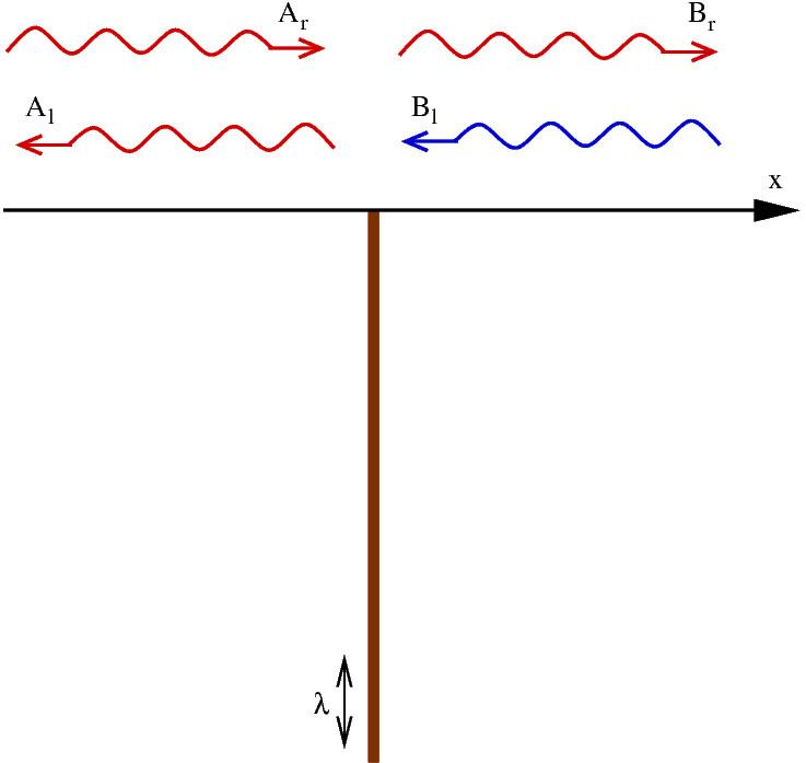
For positive energies, the particle is free to move in either half-space: x < 0 or x > 0. It may be scattered at the delta function potential.
The quantum case can be studied in the following situation: a particle incident on the barrier from the left side (Ar). It may be reflected (Al) or transmitted (Br). To find the amplitudes for reflection and transmission for incidence from the left, we put in the above equations Ar = 1 (incoming particle), Al = r (reflection), Bl = 0 (no incoming particle from the right) and Br = t (transmission), and solve for r and t even though we do not have any equations in t. The result is:
Due to the mirror symmetry of the model, the amplitudes for incidence from the right are the same as those from the left. The result is that there is a non-zero probability
for the particle to be reflected. This does not depend on the sign of λ, that is, a barrier has the same probability of reflecting the particle as a well. This is a significant difference from classical mechanics, where the reflection probability would be 1 for the barrier (the particle simply bounces back), and 0 for the well (the particle passes through the well undisturbed).
Taking this to conclusion, the probability for transmission is:
Remarks and application
The calculation presented above may at first seem unrealistic and hardly useful. However it has proved to be a suitable model for a variety of real-life systems. One such example regards the interfaces between two conducting materials. In the bulk of the materials, the motion of the electrons is quasi free and can be described by the kinetic term in the above Hamiltonian with an effective mass
The operation of a scanning tunneling microscope (STM) relies on this tunneling effect. In that case, the barrier is due to the air between the tip of the STM and the underlying object. The strength of the barrier is related to the separation being stronger the further apart the two are. For a more general model of this situation, see Finite potential barrier (QM). The delta function potential barrier is the limiting case of the model considered there for very high and narrow barriers.
The above model is one-dimensional while the space around us is three-dimensional. So in fact one should solve the Schrödinger equation in three dimensions. On the other hand, many systems only change along one coordinate direction and are translationally invariant along the others. The Schrödinger equation may then be reduced to the case considered here by an Ansatz for the wave function of the type:
Alternatively, it is possible to generalize the Dirac delta function to exist on the surface of some domain D (see Laplacian of the indicator).
The delta function model is actually a one-dimensional version of the Hydrogen atom according to the dimensional scaling method developed by the group of Dudley R. Herschbach The delta function model becomes particularly useful with the double-well Dirac Delta function model which represents a one-dimensional version of the Hydrogen molecule ion as shown in the following section.
Double delta potential
The Double-well Dirac delta function models a diatomic Hydrogen molecule by the corresponding Schrödinger equation:
where the potential is now:
where
Matching of the wavefunction at the Dirac delta function peaks yields the determinant:
Thus,
which has two solutions
The "+" case corresponds to a wave function symmetric about the midpoint (shown in red in the diagram) where
where W is the standard Lambert W function. Note that the lowest energy corresponds to the symmetric solution
One of the most interesting cases is when