Matrix multiplication

Notation

This article will use the following notational conventions: matrices are represented by capital letters in bold, e.g. A, vectors in lowercase bold, e.g. a, and entries of vectors and matrices are italic (since they are numbers from a field), e.g. A and a. Index notation is often the clearest way to express definitions, and is used as standard in the literature. The i, j entry of matrix A is indicated by (A)_ij or A_ij, whereas a numerical label (not matrix entries) on a collection of matrices is subscripted only, e.g. A₁, A₂, etc.

Matrix product (two matrices)

Assume two matrices are to be multiplied (the generalization to any number is discussed below).

General definition of the matrix product

If A is an n × m matrix and B is an m × p matrix,

the matrix product AB (denoted without multiplication signs or dots) is defined to be the n × p matrix

where each i, j entry is given by multiplying the entries A_ik (across row i of A) by the entries B_kj (down column j of B), for k = 1, 2, ..., m, and summing the results over k:

Thus the product AB is defined only if the number of columns in A is equal to the number of rows in B, in this case m. Each entry may be computed one at a time. Sometimes, the summation convention is used as it is understood to sum over the repeated index k. To prevent any ambiguity, this convention will not be used in the article.

Usually the entries are numbers or expressions, but can even be matrices themselves (see block matrix). The matrix product can still be calculated exactly the same way. See below for details on how the matrix product can be calculated in terms of blocks taking the forms of rows and columns.

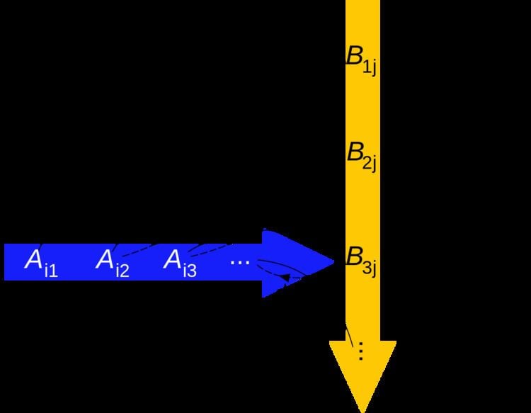
Illustration

The figure to the right illustrates diagrammatically the product of two matrices A and B, showing how each intersection in the product matrix corresponds to a row of A and a column of B.

The values at the intersections marked with circles are:

Row vector and column vector

If

their matrix products are:

and

Note AB and BA are two different matrices: the first is a 1 × 1 matrix while the second is a 3 × 3 matrix. Such expressions occur for real-valued Euclidean vectors in Cartesian coordinates, displayed as row and column matrices, in which case AB is the matrix form of their dot product, while BA the matrix form of their dyadic or tensor product.

Square matrix and column vector

If

their matrix product is:

however BA is not defined.

The product of a square matrix multiplied by a column matrix arises naturally in linear algebra; for solving linear equations and representing linear transformations. By choosing a, b, c, p, q, r, u, v, w in A appropriately, A can represent a variety of transformations such as rotations, scaling and reflections, shears, of a geometric shape in space.

Square matrices

If

their matrix products are:

and

In this case, both products AB and BA are defined, and the entries show that AB and BA are not equal in general. Multiplying square matrices which represent linear transformations corresponds to the composite transformation (see below for details).

Row vector, square matrix, and column vector

If

their matrix product is:

however CBA is not defined. Note that A(BC) = (AB)C, this is one of many general properties listed below. Expressions of the form ABC occur when calculating the inner product of two vectors displayed as row and column vectors in an arbitrary coordinate system, and the metric tensor in these coordinates written as the square matrix.

Rectangular matrices

If

their matrix products are:

and

Properties of the matrix product (two matrices)

Analogous to numbers (elements of a field), matrices satisfy the following general properties, although there is one subtlety, due to the nature of matrix multiplication.

Matrix product (any number)

Matrix multiplication can be extended to the case of more than two matrices, provided that for each sequential pair, their dimensions match.

The product of n matrices A₁, A₂, ..., A_n with sizes s₀ × s₁, s₁ × s₂, ..., s_{n − 1} × s_n (where s₀, s₁, s₂, ..., s_n are all simply positive integers and the subscripts are labels corresponding to the matrices, nothing more), is the s₀ × s_n matrix:

In index notation:

Properties of the matrix product (any number)

The same properties will hold, as long as the ordering of matrices is not changed. Some of the previous properties for more than two matrices generalize as follows.

Examples of chain multiplication

Similarity transformations involving similar matrices are matrix products of the three square matrices, in the form:

where P is the similarity matrix and A and B are said to be similar if this relation holds. This product appears frequently in linear algebra and applications, such as diagonalizing square matrices and the equivalence between different matrix representations of the same linear operator.

Operations derived from the matrix product

More operations on square matrices can be defined using the matrix product, such as powers and nth roots by repeated matrix products, the matrix exponential can be defined by a power series, the matrix logarithm is the inverse of matrix exponentiation, and so on.

Powers of matrices

Square matrices can be multiplied by themselves repeatedly in the same way as ordinary numbers, because they always have the same number of rows and columns. This repeated multiplication can be described as a power of the matrix, a special case of the ordinary matrix product. On the contrary, rectangular matrices do not have the same number of rows and columns so they can never be raised to a power. An n × n matrix A raised to a positive integer k is defined as

and the following identities hold, where λ is a scalar:

The naive computation of matrix powers is to multiply k times the matrix A to the result, starting with the identity matrix just like the scalar case. This can be improved using exponentiation by squaring, a method commonly used for scalars. For diagonalizable matrices, an even better method is to use the eigenvalue decomposition of A. Another method based on the Cayley–Hamilton theorem finds an identity using the matrices' characteristic polynomial, producing a more effective equation for A^k in which a scalar is raised to the required power, rather than an entire matrix.

A special case is the power of a diagonal matrix. Since the product of diagonal matrices amounts to simply multiplying corresponding diagonal elements together, the power k of a diagonal matrix A will have entries raised to the power. Explicitly;

meaning it is easy to raise a diagonal matrix to a power. When raising an arbitrary matrix (not necessarily a diagonal matrix) to a power, it is often helpful to exploit this property by diagonalizing the matrix first.

Linear transformations

Matrices offer a concise way of representing linear transformations between vector spaces, and matrix multiplication corresponds to the composition of linear transformations. The matrix product of two matrices can be defined when their entries belong to the same ring, and hence can be added and multiplied.

Let U, V, and W be vector spaces over the same field with given bases, S: V → W and T: U → V be linear transformations and ST: U → W be their composition.

Suppose that A, B, and C are the matrices representing the transformations S, T, and ST with respect to the given bases.

Then AB = C, that is, the matrix of the composition (or the product) of linear transformations is the product of their matrices with respect to the given bases.

Linear systems of equations

A system of linear equations with the same number of equations as variables can be solved by collecting the coefficients of the equations into a square matrix, then inverting the matrix equation.

A similar procedure can be used to solve a system of linear differential equations, see also phase plane.

The inner and outer products

Given two column vectors a and b, the Euclidean inner product and outer product are the simplest special cases of the matrix product.

Inner product

The inner product of two vectors in matrix form is equivalent to a column vector multiplied on its left by a row vector:

where a^T denotes the transpose of a.

The matrix product itself can be expressed in terms of inner product. Suppose that the first n × m matrix A is decomposed into its row vectors a_i, and the second m × p matrix B into its column vectors b_i:

where

Then:

It is also possible to express a matrix product in terms of concatenations of products of matrices and row or column vectors:

These decompositions are particularly useful for matrices that are envisioned as concatenations of particular types of row vectors or column vectors, e.g. orthogonal matrices (whose rows and columns are unit vectors orthogonal to each other) and Markov matrices (whose rows or columns sum to 1).

Outer product

The outer product (also known as the dyadic product or tensor product) of two vectors in matrix form is equivalent to a row vector multiplied on the left by a column vector:

An alternative method is to express the matrix product in terms of the outer product. The decomposition is done the other way around, the first matrix A is decomposed into column vectors a_i and the second matrix B into row vectors b_i:

where this time

This method emphasizes the effect of individual column/row pairs on the result, which is a useful point of view with e.g. covariance matrices, where each such pair corresponds to the effect of a single sample point.

Algorithms for efficient matrix multiplication

The running time of square matrix multiplication, if carried out naïvely, is O(n³). The running time for multiplying rectangular matrices (one m × p-matrix with one p × n-matrix) is O(mnp), however, more efficient algorithms exist, such as Strassen's algorithm, devised by Volker Strassen in 1969 and often referred to as "fast matrix multiplication". It is based on a way of multiplying two 2 × 2-matrices which requires only 7 multiplications (instead of the usual 8), at the expense of several additional addition and subtraction operations. Applying this recursively gives an algorithm with a multiplicative cost of O ( n log 2 ⁡ 7 ) ≈ O ( n 2.807 ) . Strassen's algorithm is more complex, and the numerical stability is reduced compared to the naïve algorithm. Nevertheless, it appears in several libraries, such as BLAS, where it is significantly more efficient for matrices with dimensions n > 100, and is very useful for large matrices over exact domains such as finite fields, where numerical stability is not an issue.

The current O(n^k) algorithm with the lowest known exponent k is a generalization of the Coppersmith–Winograd algorithm that has an asymptotic complexity of O(n^2.3728639), by François Le Gall. This algorithm, and the Coppersmith–Winograd algorithm on which it is based, are similar to Strassen's algorithm: a way is devised for multiplying two k × k-matrices with fewer than k³ multiplications, and this technique is applied recursively. However, the constant coefficient hidden by the Big O notation is so large that these algorithms are only worthwhile for matrices that are too large to handle on present-day computers.

Since any algorithm for multiplying two n × n-matrices has to process all 2 × n²-entries, there is an asymptotic lower bound of Ω(n²) operations. Raz (2002) proves a lower bound of Ω(n² log(n)) for bounded coefficient arithmetic circuits over the real or complex numbers.

Cohn et al. (2003, 2005) put methods such as the Strassen and Coppersmith–Winograd algorithms in an entirely different group-theoretic context, by utilising triples of subsets of finite groups which satisfy a disjointness property called the triple product property (TPP). They show that if families of wreath products of Abelian groups with symmetric groups realise families of subset triples with a simultaneous version of the TPP, then there are matrix multiplication algorithms with essentially quadratic complexity. Most researchers believe that this is indeed the case. However, Alon, Shpilka and Chris Umans have recently shown that some of these conjectures implying fast matrix multiplication are incompatible with another plausible conjecture, the sunflower conjecture.

Freivalds' algorithm is a simple Monte Carlo algorithm that given matrices A, B, C verifies in Θ(n²) time if AB = C.

Parallel matrix multiplication

Because of the nature of matrix operations and the layout of matrices in memory, it is typically possible to gain substantial performance gains through use of parallelization and vectorization. Several algorithms are possible, among which divide and conquer algorithms based on the block matrix decomposition

that also underlies Strassen's algorithm. Here, A, B and C are presumed to be n by n (square) matrices, and C₁₁ etc. are n/2 by n/2 submatrices. From this decomposition, one derives

which consists of eight multiplications of pairs of submatrices, which can all be performed in parallel, followed by an addition step. Applying this recursively, and performing the additions in parallel as well, one obtains an algorithm that runs in Θ(log² n) time on an ideal machine with an infinite number of processors, and has a maximum possible speedup of Θ(n³/(log² n)) on any real computer (although the algorithm isn't practical, a more practical variant achieves Θ(n²) speedup).

It should be noted that some lower time-complexity algorithms on paper may have indirect time complexity costs on real machines.

Communication-avoiding and distributed algorithms

On modern architectures with hierarchical memory, the cost of loading and storing input matrix elements tends to dominate the cost of arithmetic. On a single machine this is the amount of data transferred between RAM and cache, while on a distributed memory multi-node machine it is the amount transferred between nodes; in either case it is called the communication bandwidth. The naïve algorithm using three nested loops uses Ω(n³) communication bandwidth.

Cannon's algorithm, also known as the 2D algorithm, partitions each input matrix into a block matrix whose elements are submatrices of size √M/3 by √M/3, where M is the size of fast memory. The naïve algorithm is then used over the block matrices, computing products of submatrices entirely in fast memory. This reduces communication bandwidth to O(n³/√M), which is asymptotically optimal (for algorithms performing Ω(n³) computation).

In a distributed setting with p processors arranged in a √p by √p 2D mesh, one submatrix of the result can be assigned to each processor, and the product can be computed with each processor transmitting O(n²/√p) words, which is asymptotically optimal assuming that each node stores the minimum O(n²/p) elements. This can be improved by the 3D algorithm, which arranges the processors in a 3D cube mesh, assigning every product of two input submatrices to a single processor. The result submatrices are then generated by performing a reduction over each row. This algorithm transmits O(n²/p^2/3) words per processor, which is asymptotically optimal. However, this requires replicating each input matrix element p^1/3 times, and so requires a factor of p^1/3 more memory than is needed to store the inputs. This algorithm can be combined with Strassen to further reduce runtime. "2.5D" algorithms provide a continuous tradeoff between memory usage and communication bandwidth. On modern distributed computing environments such as MapReduce, specialized multiplication algorithms have been developed.

Other forms of multiplication

The term "matrix multiplication" is most commonly reserved for the definition given in this article. It could be more loosely applied to other definitions.