Cavity perturbation theory

General theory

When a resonant cavity is perturbed, i.e. when a foreign object with distinct material properties is introduced into the cavity or when a general shape of the cavity is changed, electromagnetic fields inside the cavity change accordingly. The underlying assumption of cavity perturbation theory is that electromagnetic fields inside the cavity after the change differ by a very small amount from the fields before the change. Then Maxwell's equations for original and perturbed cavities can be used to derive expressions for resulting resonant frequency shifts.

Cavity perturbation theory generally relies on formulae involving stored energy considerations. The following sections of this wikipedia pages are based on these formulae. The latter appear intuitive since the common sense dictates that the maximum change in resonant frequency is achieved when the small perturbation is placed at the intensity maximum of the cavity mode. This intuition is valid for high-Q cavities only and when predicting the spectral shift of the resonance frequency. However, the shift is always accompanied by a broadening of the resonance width, i.e. an increase of Q, and it is important to predict it also. The classical formulae based on energy considerations, i.e. on |E.E| products, cannot predict the broadening. For low-Q cavities, such as plasmonic resonators, they cannot predict neither the shift, nor the broadening. Correct formulae that are accurate for high- and low-Q resonators and for the shift and the brodening, have been established in 2015, see Nano Lett. 15 (5), pp 3439–3444 (2015). They are as simple, but use E.E products instead of |E.E| products. Importantly, the phase of the resonant mode is preserved in the new formulae.

Material perturbation

When a material within a cavity is changed (permittivity and/or permeability), a corresponding change in resonant frequency can be approximated as:

where ω is the angular resonant frequency of the perturbed cavity, ω 0 is the resonant frequency of the original cavity, E 0 and H 0 represent original electric and magnetic field respectively, μ and ϵ are original permeability and permittivity respectively, while Δ μ and Δ ϵ are changes in original permeability and permittivity introduced by material change.

Expression (1) can be rewritten in terms of stored energies as:

where W is the total energy stored in the original cavity and w e ¯ and w m ¯ are electric and magnetic energy densities respectively.

Shape perturbation

When a general shape of a resonant cavity is changed, a corresponding change in resonant frequency can be approximated as:

Expression (3) for change in resonant frequency can additionally be written in terms of time-average stored energies as:

where Δ W m and Δ W e represent time-average electric and magnetic energies contained in Δ V .

This expression can also be written in terms of energy densities as:

Applications

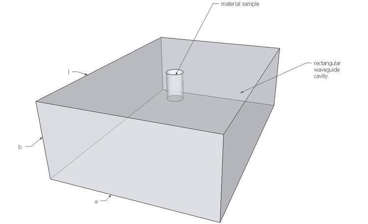
Microwave measurement techniques based on cavity perturbation theory are generally used to determine the dielectric and magnetic parameters of materials and various circuit components such as dielectric resonators. Since ex-ante knowledge of the resonant frequency, resonant frequency shift and electromagnetic fields is necessary in order to extrapolate material properties, these measurement techniques generally make use of standard resonant cavities where resonant frequencies and electromagnetic fields are well known. Two examples of such standard resonant cavities are rectangular and circular waveguide cavities and coaxial cables resonators . Cavity perturbation measurement techniques for material characterization are used in many fields ranging from physics and material science to medicine and biology.

T E 10 n {displaystyle TE_{10n}} rectangular waveguide cavity

For rectangular waveguide cavity, field distribution of dominant T E 10 n mode is well known. Ideally, the material to be measured is introduced into the cavity at the position of maximum electric or magnetic field. When the material is introduced at the position of maximum electric field, then the contribution of magnetic field to perturbed frequency shift is very small and can be ignored. In this case, we can use perturbation theory to derive expressions for real and imaginary components of complex material permittivity ϵ r = ϵ r ′ + j ϵ r ″ as:

where f c and f s represent resonant frequencies of original cavity and perturbed cavity respectively, V c and V s represent volumes of original cavity and material sample respectively, Q c and Q s represent quality factors of original and perturbed cavities respectively.

Once the complex permittivity of the material is known, we can easily calculate its effective conductivity σ e and dielectric loss tangent tan ⁡ δ as:

where f is the frequency of interest and ϵ 0 is the free space permittivity.

Similarly, if the material is introduced into the cavity at the position of maximum magnetic field, then the contribution of electric field to perturbed frequency shift is very small and can be ignored. In this case, we can use perturbation theory to derive expressions for complex material permeability μ r = μ r ′ + j μ r ″ as:

where λ g is the guide wavelength (calculated as λ g = 2 l n ).