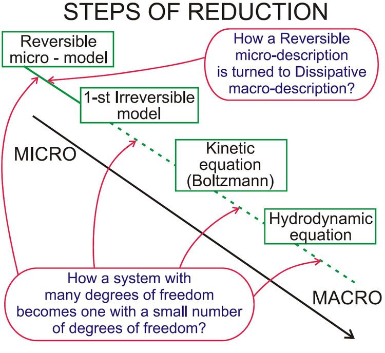
Boltzmann equation - Alchetron, The Free Social Encyclopedia

The Boltzmann equation or Boltzmann transport equation (BTE) describes the statistical behaviour of a thermodynamic system not in a state of equilibrium, devised by Ludwig Boltzmann in 1872. The classic example of such a system is a fluid with temperature gradients in space causing heat to flow from hotter regions to colder ones, by the random but biased transport of the particles making up that fluid. In the modern literature the term Boltzmann equation is often used in a more general sense, referring to any kinetic equation that describes the change of a macroscopic quantity in a thermodynamic system, such as energy, charge or particle number.

The equation arises not by analyzing the individual positions and momenta of each particle in the fluid but rather by considering a probability distribution for the position and momentum of a typical particle—that is, the probability that the particle occupies a given very small region of space (mathematically written d 3 r , where d means "differential") centered at the position r , and has momentum nearly equal to a given momentum vector p (thus occupying a very small region of momentum space d 3 p ), at an instant of time.

The Boltzmann equation can be used to determine how physical quantities change, such as heat energy and momentum, when a fluid is in transport. One may also derive other properties characteristic to fluids such as viscosity, thermal conductivity, and electrical conductivity (by treating the charge carriers in a material as a gas). See also convection-diffusion equation.

The equation is a nonlinear integro-differential equation, and the unknown function in the equation is a probability density function in six-dimensional space of a particle position and momentum. The problem of existence and uniqueness of solutions is still not fully resolved, but some recent results are quite promising.

The phase space and density function

The set of all possible positions r and momenta p is called the phase space of the system; in other words a set of three coordinates for each position coordinate x, y, z, and three more for each momentum component p_x, p_y, p_z. The entire space is 6-dimensional: a point in this space is (r, p) = (x, y, z, p_x, p_y, p_z), and each coordinate is parameterized by time t. The small volume ("differential volume element") is written

d 3 r d 3 p = d x d y d z d p x d p y d p z .

Since the probability of N molecules which all have r and p within d 3 r d 3 p is in question, at the heart of the equation is a quantity f which gives this probability per unit phase-space volume, or probability per unit length cubed per unit momentum cubed, at an instant of time t. This is a probability density function: f(r, p, t), defined so that,

d N = f ( r , p , t ) d 3 r d 3 p

is the number of molecules which all have positions lying within a volume element d 3 r about r and momenta lying within a momentum space element d 3 p about p, at time t. Integrating over a region of position space and momentum space gives the total number of particles which have positions and momenta in that region:

N = ∫ p o s i t i o n s d 3 r ∫ m o m e n t a d 3 p f ( r , p , t ) = ∭ p o s i t i o n s ∭ m o m e n t a f ( x , y , z , p x , p y , p z , t ) d x d y d z d p x d p y d p z

which is a 6-fold integral. While f is associated with a number of particles, the phase space is for one-particle (not all of them, which is usually the case with deterministic many-body systems), since only one r and p is in question. It is not part of the analysis to use r₁, p₁ for particle 1, r₂, p₂ for particle 2, etc. up to r_N, p_N for particle N.

It is assumed the particles in the system are identical (so each has an identical mass m). For a mixture of more than one chemical species, one distribution is needed for each, see below.

Principal statement

The general equation can then be written:

∂ f ∂ t = ( ∂ f ∂ t ) f o r c e + ( ∂ f ∂ t ) d i f f + ( ∂ f ∂ t ) c o l l

where the "force" term corresponds to the forces exerted on the particles by an external influence (not by the particles themselves), the "diff" term represents the diffusion of particles, and "coll" is the collision term – accounting for the forces acting between particles in collisions. Expressions for each term on the right side are provided below.

Note that some authors use the particle velocity v instead of momentum p; they are related in the definition of momentum by p = mv.

The force and diffusion terms

Consider particles described by f, each experiencing an external force F not due to other particles (see the collision term for the latter treatment).

Suppose at time t some number of particles all have position r within element d 3 r and momentum p within d 3 p . If a force F instantly acts on each particle, then at time t + Δt their position will be r + Δr = r + pΔt/m and momentum p + Δp = p + FΔt. Then, in the absence of collisions, f must satisfy

f ( r + p m Δ t , p + F Δ t , t + Δ t ) d 3 r d 3 p = f ( r , p , t ) d 3 r d 3 p

Note that we have used the fact that the phase space volume element d 3 r d 3 p is constant, which can be shown using Hamilton's equations (see the discussion under Liouville's theorem). However, since collisions do occur, the particle density in the phase-space volume d 3 r ' d 3 p changes, so

where Δf is the total change in f. Dividing (1) by d 3 r d 3 p Δt and taking the limits Δt → 0 and Δf → 0, we have

The total differential of f is:

where ∇ is the gradient operator, · is the dot product,

∂ f ∂ p = e ^ x ∂ f ∂ p x + e ^ y ∂ f ∂ p y + e ^ z ∂ f ∂ p z = ∇ p f

is a shorthand for the momentum analogue of ∇, and ê_x, ê_y, ê_z are Cartesian unit vectors.

Final statement

Dividing (3) by dt and substituting into (2) gives:

∂ f ∂ t + p m ⋅ ∇ f + F ⋅ ∂ f ∂ p = ( ∂ f ∂ t ) c o l l

In this context, F(r, t) is the force field acting on the particles in the fluid, and m is the mass of the particles. The term on the right hand side is added to describe the effect of collisions between particles; if it is zero then the particles do not collide. The collisionless Boltzmann equation is often called the Vlasov equation.

This equation is more useful than the principal one above, yet still incomplete, since f cannot be solved unless the collision term in f is known. This term cannot be found as easily or generally as the others – it is a statistical term representing the particle collisions, and requires knowledge of the statistics the particles obey, like the Maxwell–Boltzmann, Fermi–Dirac or Bose–Einstein distributions.

The collision term (Stosszahlansatz) and molecular chaos

A key insight applied by Boltzmann was to determine the collision term resulting solely from two-body collisions between particles that are assumed to be uncorrelated prior to the collision. This assumption was referred to by Boltzmann as the "Stosszahlansatz", and is also known as the "molecular chaos assumption". Under this assumption the collision term can be written as a momentum-space integral over the product of one-particle distribution functions:

( ∂ f ∂ t ) c o l l = ∬ g I ( g , Ω ) [ f ( p ′ A , t ) f ( p ′ B , t ) − f ( p A , t ) f ( p B , t ) ] d Ω d 3 p A d 3 p B .

where p_A and p_B are the momenta of any two particles (labeled as A and B for convenience) before a collision, p′_A and p′_B are the momenta after the collision,

g = | p B − p A | = | p ′ B − p ′ A |

is the magnitude of the relative momenta (see relative velocity for more on this concept), and I(g, Ω) is the differential cross section of the collision, in which the relative momenta of the colliding particles turns through an angle θ into the element of the solid angle dΩ, due to the collision.

Simplifications to the Boltzmann equation collision term

Since much of the challenge in solving the Boltzmann equation originates with the complex collision term, attempts have been made to 'model' and simplify the collision term. The best known model equation is due to Bhatnagar, Gross and Krook. The assumption in the BGK approximation is that the effect of molecular collisions is to force a non-equilibrium distribution function at a point in physical space back to a Maxwellian equilibrium distribution function and that the rate at which this occurs is proportional to the molecular collision frequency. The Boltzmann equation is therefore modified to the BGK form,

∂ f ∂ t + p m ⋅ ∇ f + F ⋅ ∂ f ∂ p = ν ( f 0 − f )

where ν is the molecular collision frequency and f 0 is the local Maxwellian distribution function given the gas temperature at this point in space.

General equation (for a mixture)

For a mixture of chemical species labelled by indices i = 1,2,3...,n the equation for species i is:

∂ f i ∂ t + p i m i ⋅ ∇ f i + F ⋅ ∂ f i ∂ p i = ( ∂ f i ∂ t ) c o l l

where f_i = f_i(r, p_i, t), and the collision term is

( ∂ f i ∂ t ) c o l l = ∑ j = 1 n ∬ g i j I i j ( g i j , Ω ) [ f i ′ f j ′ − f i f j ] d Ω d 3 p ′ .

where f′ = f′(p′_i, t), the magnitude of the relative momenta is

g i j = | p i − p j | = | p ′ i − p ′ j |

and I_ij is the differential cross-section as before, between particles i and j. The integration is over the momentum components in the integrand (which are labelled i and j). The sum of integrals describes the entry and exit of particles of species i in or out of the phase space element.

Conservation equations

The Boltzmann equation can be used to derive the fluid dynamic conservation laws for mass, charge, momentum and energy. For a fluid consisting of only one kind of particle, the number density n is given by:

n = ∫ f d 3 p

The average value of any function A is:

⟨ A ⟩ = 1 n ∫ A f d 3 p

Since the conservation equations involve tensors, the Einstein summation convention will be used where repeated indices in a product indicate summation over those indices. Thus x → x i and p → p i = m w i where w i is the particle velocity vector. Define g ( p i ) as some function of momentum p i only, which is conserved in a collision. Assume also that the force F i is a function of position only, and that f is zero for p i → ± ∞ . Multiplying the Boltzmann equation by g and integrating over momentum yields four terms which, using integration by parts, can be expressed as:

∫ g ∂ f ∂ t d 3 p = ∂ ∂ t ( n ⟨ g ⟩ ) ∫ p j g m ∂ f ∂ x j d 3 p = 1 m ∂ ∂ x j ( n ⟨ g p j ⟩ ) ∫ g F j ∂ f ∂ p j d 3 p = − n F j ⟨ ∂ g ∂ p j ⟩ ∫ g ( ∂ f ∂ t ) c o l l d 3 p = 0

where the last term is zero since g is conserved in a collision. Letting g = m , the mass of the particle, the integrated Boltzmann equation becomes the conservation of mass equation:

∂ ∂ t ρ + ∂ ∂ x j ( ρ V j ) = 0

where ρ = m n is the mass density and V i = ⟨ w i ⟩ is the average fluid velocity.

Letting g = m w i , the momentum of the particle, the integrated Boltzmann equation becomes the conservation of momentum equation:

∂ ∂ t ( ρ V i ) + ∂ ∂ x j ( ρ V i V j + P i j ) − n F i = 0

where P i j = ρ ⟨ ( w i − V i ) ( w j − V j ) ⟩ is the pressure tensor. (The viscous stress tensor plus the hydrostatic pressure.)

Letting g = 1 2 m w i w i , the kinetic energy of the particle, the integrated Boltzmann equation becomes the conservation of energy equation:

∂ ∂ t ( u + 1 2 ρ V i V i ) + ∂ ∂ x j ( u V j + 1 2 ρ V i V i V j + J q j + P i j V i ) − n F i V i = 0

where u = 1 2 ρ ⟨ ( w i − V i ) ( w i − V i ) ⟩ is the kinetic thermal energy density and J q i = 1 2 ρ ⟨ ( w i − V i ) ( w k − V k ) ( w k − V k ) ⟩ is the heat flux vector.

Hamiltonian mechanics

In Hamiltonian mechanics, the Boltzmann equation is often written more generally as

L ^ [ f ] = C [ f ] ,

where L is the Liouville operator describing the evolution of a phase space volume and C is the collision operator. The non-relativistic form of L is

L ^ N R = ∂ ∂ t + p m ⋅ ∇ + F ⋅ ∂ ∂ p .

Quantum theory and violation of particle number

It is possible to write down relativistic Boltzmann equations for relativistic quantum systems in which the number of particles is not conserved in collisions. This has several applications in physical cosmology, including the formation of the light elements in big bang nucleosynthesis, the production of dark matter and baryogenesis. It is not a priori clear that the state of a quantum system can be characterized by a classical phase space density f. However, for a wide class of applications a well-defined generalization of f exists which is the solution of an effective Boltzmann equation that can be derived from first principles of quantum field theory.

General relativity and astronomy

The Boltzmann equation is of use in galactic dynamics. A galaxy, under certain assumptions, may be approximated as a continuous fluid; its mass distribution is then represented by f; in galaxies, physical collisions between the stars are very rare, and the effect of gravitational collisions can be neglected for times far longer than the age of the universe.

Its generalization in general relativity is

L ^ G R = p α ∂ ∂ x α − Γ α β γ p β p γ ∂ ∂ p α ,

where Γ^α_βγ is the Christoffel symbol of the second kind (this assumes there are no external forces, so that particles move along geodesics in the absence of collisions), with the important subtlety that the density is a function in mixed contravariant-covariant (xⁱ, p_i) phase space as opposed to fully contravariant (xⁱ, pⁱ) phase space.

In physical cosmology, the study of processes in the early universe often requires to take into account the effects of quantum mechanics and general relativity. In the very dense medium formed by the primordial plasma after the big bang, particles are continuously created and annihilated. In such an environment quantum coherence and the spatial extension of the wavefunction can affect the dynamics, making it questionable whether the classical phase space distribution f that appears in the Boltzmann equation is suitable to describe the system. In many cases it is, however, possible to derive an effective Boltzmann equation for a generalized distribution function from first principles of quantum field theory. This includes the formation of the light elements in big bang nucleosynthesis, the production of dark matter and baryogenesis.

Solutions to the Boltzmann equation

It was proven only in 2010 that exact solutions to the Boltzmann equation are always mathematically well-behaved. This means that if a system obeying the Boltzmann equation is perturbed, then it will return to equilibrium, rather than diverging to infinity or behaving otherwise. However, this existence proof is not helpful for solving the equation in realistic scenarios. Indeed, such statements only tell us whether the solution subject to specified conditions exist, but not how to find them. In practice, numerical methods are used to find approximate solutions to the various forms of the Boltzmann equation with applications ranging from hypersonic aerodynamics in rarefied gas flows to plasma flows.

References

Boltzmann equation Wikipedia

(Text) CC BY-SA

Contents