Angular momentum diagrams (quantum mechanics) - Alchetron, the free social encyclopedia

In quantum mechanics and its applications to quantum many-particle systems, notably quantum chemistry, angular momentum diagrams, or more accurately from a mathematical viewpoint angular momentum graphs, are a diagrammatic method for representing angular momentum quantum states of a quantum system allowing calculations to be done symbolically. More specifically, the arrows encode angular momentum states in bra–ket notation and include the abstract nature of the state, such as tensor products and transformation rules.

The notation parallels the idea of Penrose graphical notation and Feynman diagrams. The diagrams consist of arrows and vertices with quantum numbers as labels, hence the alternative term "graphs". The sense of each arrow is related to Hermitian conjugation, which roughly corresponds to time reversal of the angular momentum states (c.f. Schrödinger equation). The diagrammatic notation is a considerably large topic in its own right with a number of specialized features – this article introduces the very basics.

They were developed primarily by Adolfas Jucys in the twentieth century.

Angular momentum states

The quantum state vector of a single particle with total angular momentum quantum number j and total magnetic quantum number m = j, j − 1, ..., −j + 1, −j, is denoted as a ket |j, m⟩. As a diagram this is a singleheaded arrow.

Symmetrically, the corresponding bra is ⟨j, m|. In diagram form this is a doubleheaded arrow, pointing in the opposite direction to the ket.

In each case;

the quantum numbers j, m are often labelled next to the arrows to refer to a specific angular momentum state,

arrowheads are almost always placed at the middle of the line, rather than at the tip,

equals signs "=" are placed between equivalent diagrams, exactly like for multiple algebraic expressions equal to each other.

The most basic diagrams are for kets and bras:

Arrows are directed to or from vertices, a state transforming according to:

a standard representation is designated by an oriented line leaving a vertex,

a contrastandard representation is depicted as a line entering a vertex.

As a general rule, the arrows follow each other in the same sense. In the contrastandard representation, the time reversal operator, denoted here by T, is used. It is unitary, which means the Hermitian conjugate T^† equals the inverse operator T⁻¹, that is T^† = T⁻¹. It's action on the position operator leaves it invariant:

T x ^ T † = x ^

but the linear momentum operator becomes negative:

T p ^ T † = − p ^

and the spin operator becomes negative:

T S ^ T † = − S ^

Since the orbital angular momentum operator is L = x × p, this must also become negative:

T L ^ T † = − L ^

and therefore the total angular momentum operator J = L + S becomes negative:

T J ^ T † = − J ^

Acting on an eigenstate of angular momentum |j, m⟩, it can be shown that [see for example P.E.S. Wormer and J. Paldus (2006)]:

T | j , m ⟩ ≡ | T ( j , m ) ⟩ = ( − 1 ) j − m | j , − m ⟩

The time-reversed diagrams for kets and bras are:

It is important to position the vertex correctly, as forward-time and reversed-time operators would become mixed up.

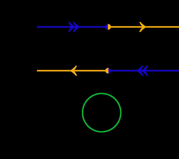
Inner product

The inner product of two states |j₁, m₁⟩ and |j₂, m₂⟩ is:

⟨ j 2 , m 2 | j 1 , m 1 ⟩ = δ j 1 j 2 δ m 1 m 2

and the diagrams are:

For summations over the inner product, also known in this context as a contraction (c.f. tensor contraction):

∑ m ⟨ j , m | j , m ⟩ = 2 j + 1

it is conventional to denote the result as a closed circle labelled only by j, not m:

Outer products

The outer product of two states |j₁, m₁⟩ and |j₂, m₂⟩ is an operator:

| j 2 , m 2 ⟩ ⟨ j 1 , m 1 |

and the diagrams are:

For summations over the outer product, also known in this context as a contraction (c.f. tensor contraction):

∑ m | j , m ⟩ ⟨ j , m | = ∑ m | j , − m ⟩ ⟨ j , − m | = ∑ m ( − 1 ) 2 ( j − m ) | j , − m ⟩ ⟨ j , − m | = ∑ m ( − 1 ) j − m | j , − m ⟩ ⟨ j , − m | ( − 1 ) j − m = ∑ m T | j , m ⟩ ⟨ j , m | T †

where the result for T|j, m⟩ was used, and the fact that m takes the set of values given above. There is no difference between the forward-time and reversed-time states for the outer product contraction, so here they share the same diagram, represented as one line without direction, again labelled by j only and not m:

Tensor products

The tensor product ⊗ of n states |j₁, m₁⟩, |j₂, m₂⟩, ... |j_n, m_n⟩ is written

| j 1 , m 1 , j 2 , m 2 , . . . j n , m n ⟩ ≡ | j 1 , m 1 ⟩ ⊗ | j 2 , m 2 ⟩ ⊗ ⋯ ⊗ | j n , m n ⟩ ≡ | j 1 , m 1 ⟩ | j 2 , m 2 ⟩ ⋯ | j n , m n ⟩

and in diagram form, each separate state leaves or enters a common vertex creating a "fan" of arrows - n lines attached to a single vertex.

Vertices in tensor products have signs (sometimes called "node signs"), to indicate the ordering of the tensor-multiplied states:

a minus sign (−) indicates the ordering is clockwise, ↻ , and

a plus sign (+) for anticlockwise, ↺ .

Signs are of course not required for just one state, diagrammatically one arrow at a vertex. Sometimes curved arrows with the signs are included to show explicitly the sense of tensor multiplication, but usually just the sign is shown with the arrows left out.

For the inner product of two tensor product states:

⟨ j n ′ , m n ′ , . . . , j 2 ′ , m 2 ′ , j 1 ′ , m 1 ′ | j 1 , m 1 , j 2 , m 2 , . . . j n , m n ⟩ = ⟨ j n ′ , m n ′ | . . . ⟨ j 2 ′ , m 2 ′ | ⟨ j 1 ′ , m 1 ′ | | j 1 , m 1 ⟩ | j 2 , m 2 ⟩ . . . | j n , m n ⟩ = ∏ k = 1 n ⟨ j k ′ , m k ′ | j k , m k ⟩

there are n lots of inner product arrows:

Examples and applications

The diagrams are well-suited for Clebsch–Gordan coefficients.

Calculations with real quantum systems, such as multielectron atoms and molecular systems.

References

Angular momentum diagrams (quantum mechanics) Wikipedia

(Text) CC BY-SA